Bittner (2002a) uses a BSP tree to calculate and represent the visibility map. ... common to calculate visibility for a group of triangles .... The visibility channel stores the percentage .... rectly handle CSG models, parametric and implicit sur- faces ...
Visibility in Computer Graphics Jiˇr´ı Bittner†§ and Peter Wonka§‡ †
Center for Applied Cybernetics Czech Technical University in Prague § Institute of Computer Graphics and Algorithms Vienna University of Technology ‡ Graphics, Visualization, and Usability Center Georgia Institute of Technology
Abstract
or surfaces are visible in a synthesized image of a 3D scene. These problems are known as visible line and visible surface determination or as hidden line and hidden surface removal. The classical visible line and visible surface algorithms were developed in the early days of computer graphics in the late 60’s and the beginning of the 70’s (Sutherland et al., 1974). These techniques were mostly designed for vector displays. Later, with increasing availability of raster devices the traditional techniques were replaced by the z-buffer algorithm (Catmull, 1975). Nowadays, we can identify two widely spread visibility algorithms: the z-buffer for visible surface determination and ray shooting for computing visibility along a single ray. The z-buffer and its modifications dominate the area of real-time rendering whereas ray shooting is commonly used in the scope of global illumination methods. Besides these two elementary methods there is a plethora of visibility algorithms for various specific visibility problems. Several surveys of visibility methods have been published. The classical survey of Sutherland, Sproull, and Schumacker (1974) covers ten traditional visible surface algorithms. This survey was updated by Grant (1992) who provides a classification of visibility algorithms that includes newer rendering paradigms such as distributed ray tracing. A survey of Durand (1999) provides a comprehensive multidisciplinary overview of visibility techniques in various research areas. A recent survey of Cohen-Or et al. (2002) summarizes visibility algorithms for walkthrough applications. In this paper we aim to provide a new taxonomy of visibility problems encountered in computer graphics
Visibility computation is crucial for computer graphics from its very beginning. The first visibility algorithms in computer graphics aimed to determine visible surfaces in a synthesized image of a 3D scene. Nowadays there are many different visibility algorithms for various visibility problems. We propose a new taxonomy of visibility problems that is based on a classification according to the problem domain. We provide a broad overview of visibility problems and algorithms in computer graphics grouped by the proposed taxonomy. The paper surveys visible surface algorithms, visibility culling algorithms, visibility algorithms for shadow computation, global illumination, point-based and image-based rendering, and global visibility computations. Finally, we discuss common concepts of visibility algorithm design and several criteria for the classification of visibility algorithms.
1
Introduction
Visibility is studied in computer graphics, architecture, computational geometry, computer vision, robotics, telecommunications, and other research areas. In this paper we discuss visibility problems and algorithms from the point of view of computer graphics. Computer graphics aims to synthesize images of virtual scenes by simulating the propagation of light. Visibility is a crucial phenomenon that is an integral part of the interaction of light with the environment. The first visibility algorithms aimed to determine which lines 1
The domain description is independent of the dimension of the scene, i.e. the problem of visibility from a point can be stated for 2D, 2 21 D, and 3D scenes. The actual domains however differ depending on the scene dimension. For example, as we shall see later, visibility from a polygon is equivalent to visibility from a region in 2D, but not in 3D. The problem domains can further be categorized as discrete or continuous. A discrete domain consists of a finite set of lines (rays), which is a common situation when the problem aims at computing visibility with respect to a raster image.
based on the problem domain. The taxonomy should help to understand the nature of a particular visibility problem and provides a tool for grouping problems of similar complexity independently of their target application. We provide a broad overview of visibility problems and algorithms in computer graphics grouped by the proposed taxonomy. The paper surveys visible surface algorithms, visibility culling algorithms for, visibility algorithms for shadow computation, global illumination, point-based and image-based rendering, and global visibility computations. In contrast to the previous surveys, we focus on the common ideas and concepts rather than algorithmic details. We aim to assist a potential algorithm designer in transferring the concepts developed in the computer graphics community to solve visibility problems in other research areas.
2
2.1.1 The dimension of visibility problems We assume that a line in primal space can be mapped to a point in line space (Stolfi, 1991; Pellegrini, 1997; Teller, 1992b; Durand, 1999). In 3D there are four degrees of freedom in the description of a line and thus the corresponding line space is four-dimensional. Fixing certain line parameters (e.g. direction), the problemrelevant line set, denoted L3x , forms a k-dimensional subset of R4 , where 0 ≤ k ≤ 4. The superscript (3) expresses the dimension of primal space, the subscript (x) corresponds to one of the problem domain classes: l for visibility along a line, p for visibility from a point, s for visibility from a line segment, n for visibility from a polygon, r for visibility from a region, and g for global visibility. In 2D there are two degrees of freedom in the description of a line and the corresponding line space is two-dimensional. Therefore, the problem-relevant line set L2x forms a k-dimensional subset of R2 , where 0 ≤ k ≤ 2. An illustration of the concept of the problem-relevant line set is depicted in Figure 1. For the purpose of this discussion we define the dimension of the visibility problem as the dimension of the corresponding problem-relevant line set.
Taxonomy of visibility problems
Visibility is a phenomenon that can be defined by means of mutually unoccluded points: two points are mutually visible if the line segment connecting them is unoccluded. From this definition we can make two observations: (1) lines carry visibility, (2) two points can be visible regardless of their distance. The first observation says that the domain of a visibility problem is formed by the set of lines through which the scene entities might be visible. We call this set the problem-relevant line set. The second observation says that visibility of scene entities is independent of their spatial proximity.
2.1
Problem domain
The problem domain is given by the problem-relevant line set, i.e. by the set of lines involved in the solution of the problem. Computer graphics deals with the following domains:
2.2
1. visibility along a line
Visibility along a line
The simplest visibility problems deal with visibility along a single line. The problem-relevant line set is zero-dimensional, i.e. it is fully specified by the given line. The visibility along a line problems can be solved by computing intersections of the given line with the scene objects. The most common visibility along a line problem is ray shooting (Arvo & Kirk, 1989). Given a ray, ray shooting determines the first intersection of the ray with
2. visibility from a point 3. visibility from a line segment 4. visibility from a polygon 5. visibility from a region 6. global visibility 2
visibility along a line
visibility from a point
visibility from a segment
Figure 1: Problem-relevant line sets in 2D. L2l corresponds to a single point that is a mapping of the given line. L2p is formed by points lying on a line. This line is a dual mapping of the point p. L2s is formed by a 2D subset induced by the intersection of dual mappings of endpoints of the given segment. a scene object. A similar problem to ray shooting is point-to-point visibility. Point-to-point visibility determines whether the line segment between two points is unoccluded, i.e. the line segment has no intersection with an opaque object in the scene. Another visibility along a line problem is determining the maximal free line segments on a given line. See Figure 2 for an illustration of typical visibility along a line problems.
viewing plane
view point
y x
2.3
Visibility from a point
Lines intersecting a point in 3D can be described by two parameters. For example the lines can be expressed by an intersection with a unit sphere centered at the given point. The most common parametrization describes a line by a point of intersection with a (viewing) plane (see Figure 3). In 3D the problem-relevant line set L3p is a 2D subset of the 4D line space. In 2D L2p is a 1D subset of the 2D line space. Thus to solve visibility from a point in 3D (2D) accurately we need to account for visibility along each line of the 2D (1D) set.
Figure 3: Visibility from a point. Lines intersecting a point can be described by a point of intersection with a plane. The typical visibility from a point problem is visible surface determination (Foley et al., 1990). Due to its importance for image synthesis visible surface determination covers the majority of existing visibility algorithms in computer graphics. The problem of point-to-region visibility aims to classify a region as vis3
B
B
invisible A
A
A
Figure 2: Visibility along a line. (left) Ray shooting. (center) Point-to-point visibility. (right) Maximal free line segments between two points. ible, invisible, or partially visible with respect to the given point (Teller & S´equin, 1991). Another visibility from a point problem is the construction of the visibility map (Stewart & Karkanis, 1998), i.e. a graph describing the given view of the scene including its topology.
The segment-to-region visibility (Wonka et al., 2000) is used for visibility preprocessing in 2 12 D scenes. Visibility from a line segment also arises in the computation of soft shadows due to a linear light source (Heidrich et al., 2000).
2.4
2.5
Visibility from a line segment
In 3D, lines intersecting a polygon can be described by four parameters (Gu et al., 1997; Pellegrini, 1997). For example: two parameters fix a point inside the polygon, the other two parameters describe a direction of the line. We can imagine L3n as a 2D set of L3p associated with all points inside the polygon (see Figure 4). L3n is a four-dimensional subset of the 4D line space. In 2D, lines intersecting a polygon consists of sets that intersect the boundary line segments of the polygon and thus L2n is two-dimensional. Visibility from a polygon problems include computing a form-factor between two polygons (Goral et al., 1984), soft shadow algorithms (Chin & Feiner, 1992), and discontinuity meshing (Heckbert, 1992).
Lines intersecting a line segment in 3D can be described by three parameters. One parameter fixes the intersection of the line with the segment the other two express the direction of the line. Thus we can image Lxs as a 1D set of Lxp that are associated with all points on the given segment (see Figure 4). The problemrelevant line set L3s is three-dimensional and L2s is twodimensional. An interesting observation is that in 2D, visibility from a line segment already reaches the dimension of the whole line space. segment
plane
line space
occluded lines
1
object u
L0
0.5
L0
L0.5
0
2.6 Visibility from a region
L0.5 y
L1 x
y
u
L1
x
0
Visibility from a polygon
0.5
1
Figure 4: Visibility from a line segment. Lines intersecting a line segment form L3s . The figure shows a possible parametrization that stacks up 2D planes. Each plane corresponds to mappings of lines intersecting a point on the given line segment. 4
Lines intersecting a volumetric region in 3D can be described by four parameters. Similarly to the case of lines intersecting a polygon two parameters can fix a point on the boundary of the region, the other two fix the direction of the line. Thus L3r is four-dimensional and the corresponding visibility problems belong to the same complexity class as the from-polygon visibility problems. In 2D, visibility from a 2D region is equivalent to visibility from a polygon: L2r is a 2D subset of 2D line space.
to those of visibility from a region problems there is no given set of reference points from which visibility is studied and thus there is no given priority ordering of objects along each particular line. Therefore an additional parameter must be used to describe visibility (e.g. visible objects) along each ray. Additionally, the global visibility problems typically deal with a much larger sets of rays. Global visibility problems include view space partitioning (Plantinga et al., 1990), computation of the visibility complex (Pocchiola & Vegter, 1993), or visibility skeleton (Durand et al., 1997).
2.8
Figure 5: Visibility from a polygon. The figure depicts boundary rays of line sets through which the three polygons are visible.
Summary
The summary of the taxonomy of visibility problems is given in Table 1. The classification according to the dimension of the problem-relevant line set provides A typical visibility from a region problem is the means for understanding how difficult it is to compute problem of region-to-region visibility (Teller & S´equin, and maintain visibility for a particular class of prob1991) that aims to determine if the two given regions lems. For example a data structure representing the visiin the scene are mutually visible, invisible or partially ble or occluded parts of the scene for the visibility from 3 visible (see Figure 6). The region-to-region visibility a point problem needs to partition 2D Lp into visible problem arises in the context of computing a potentially and occluded sets of lines. This observation conforms visible set (PVS), i.e. the set of objects potentially visi- with the traditional visible surface algorithms that partition an image into empty/nonempty regions and assoble from any point inside the given region. ciate each nonempty region (pixel) with a visible object. primal space line space In this case the image represents L3p as each point of the image corresponds to a line through that point. To analytically describe visibility from a region a subdiviA* sion of 4D L3r should be performed. This is much more A difficult than the 2D subdivision. Moreover the description of visibility from a region involves non-linear subB* divisions of both primal space and line space even for B polygonal scenes (Teller, 1992a; Durand, 1999). The classification also shows that solutions to many visibility problems in 2D do not extend easily to 3D since Figure 6: Region-to-region visibility. Two regions and they involve line sets of different dimensions (Durand, two occluders in a 2D scene. In line space the region- 1999). to-region visibility can be solved by subtracting the set of lines intersecting objects A and B from lines intersecting both regions.
3
2.7
Global visibility
Visibility problems and algorithms
This section provides an overview of representative visibility problems and algorithms. We do not aim to give detailed descriptions of the algorithms. Instead we provide a catalog of visibility algorithms structured according to the taxonomy. Within each class of the taxonomy
Global visibility problems pose no restrictions on the problem-relevant line set as they consider all lines in the scene. Thus L3g is four-dimensional and L2g is twodimensional. Although these dimensions are equivalent 5
problem domain
2D
dimension of Lyx
visibility along a line
0
visibility from a point
1
visibility from a line segment visibility from a polygon visibility from a region global visibility
2
visibility along a line
0
visibility from a point
2
visibility from a line segment
3
visibility from a polygon visibility from a region global visibility
4
3D
common problems ray shooting point-to-point visibility view around a point point-to-region visibility region-to-region visibility PVS ray shooting point-to-point visibility visible (hidden) surfaces point-to-region visibility visibility map hard shadows segment-to-region visibility soft shadows PVS in 2 12 D scenes region-to-region visibility PVS aspect graph soft shadows discontinuity meshing
Table 1: Classification of visibility problems according to the dimension of the problem-relevant line set. the algorithms are grouped according to the actual visibility problem or important algorithmic features.
3.1
was presented by Havran (2000).
Visibility along a line
Point-to-point visibility Point-to-point visibility is used within the ray tracing algorithm (Whitted, 1979) to Ray shooting Ray shooting is the most common vis- test whether a given point is in shadow with respect to ibility along a line problem. Given a ray, ray shooting a point light source. This query is typically resolved by determines the first intersection of the ray with a scene casting shadow rays from the given point towards the object. Ray shooting was first used by Appel (1968) to light source. This process can be accelerated by presolve the visible surface problem for each pixel of the processing visibility from the light source (Haines & image. Ray shooting is the core of the ray tracing algo- Greenberg, 1986; Woo & Amanatides, 1990) (see Secrithm (Whitted, 1979) that follows light paths from the tion 3.2.5 for more details). view point backwards to the scene. Many recent methods use ray shooting driven by stochastic sampling for more accurate simulation of light propagation (Kajiya, 1986; Arvo & Kirk, 1990). A naive ray shooting algo- 3.2 Visibility from a point rithm tests all objects for intersection with a given ray to find the closest visible object along the ray in Θ(n) Visibility from a point problems cover the majority of time (where n is the number of objects). For complex visibility algorithms developed in the computer graphscenes even the linear time complexity is very restric- ics community. We subdivide this section according to tive since a huge amount of rays is needed to synthesize five subclasses: visible surface determination, visibility an image. An overview of acceleration techniques for culling, hard shadows, global illumination, and imageray shooting was given by Arvo (1989). A recent survey based and point-based rendering. 6
3.2.1
Visible surface determination
seen from an arbitrary view point. Improved outputsensitive variants of the algorithm generate a front-toback order of polygons and an image space data structure for correct image updates (Gordon & Chen, 1991; Naylor, 1992).
Visible surface determination aims to determine visible surfaces in the synthesized image, which is the most common visibility problem in computer graphics. Z-buffer The z-buffer, introduced by Catmull (1975), is one of the simplest visible surface algorithms. Its simplicity allows an efficient hardware implementation and therefore the z-buffer is nowadays commonly available even on low cost graphics hardware. The z-buffer is a discrete algorithm that associates a depth value with each pixel of the image. The z-buffer performs discrete sampling of visibility and therefore the rendering algorithms based on the z-buffer are prone to aliasing (Carpenter, 1984). The z-buffer algorithm is not output sensitive since it needs to rasterize all scene objects even if many objects are invisible. This is not restrictive for scenes where most of the scene elements are visible, such as a single albeit complex object. For large scenes with high depth complexity the processing of invisible objects causes significant overdraw. Overdraw expresses how many polygons are rasterized at a pixel (only the closest polygon is actually visible). The overdraw problem is addressed by visibility culling methods that will be discussed in Section 3.2.4.
Area subdivision algorithms Warnock (1969) developed an area subdivision algorithm that subdivides a given image area into four rectangles. In the case that visibility within the current rectangle cannot be solved, the rectangle is recursively subdivided. The subdivision is terminated when the area matches the pixel size. The algorithm of Weiler and Atherton (1977) subdivides the image plane using the actual polygon boundaries. The algorithm does not rely on a pixel resolution but it requires a robust polygon clipping algorithm. Scan line algorithms The scan-line visibility algorithms extend the scan conversion of a single polygon (Foley et al., 1990). They maintain an active edge table that indicates which polygons span the current scan line. The scan line coherence is exploited using incremental updates of the active edge table similarly to the scan conversion of a single polygon. Ray casting Ray casting (Appel, 1968) is a visible surface algorithm that solves visibility by ray shooting. More specifically by shooting rays through each pixel in the image. The advantage of ray casting is that it is inherently output sensitive (Wald et al., 2001).
List priority algorithms List priority algorithms determine an ordering of scene objects so that a correct image is produced if the objects are rendered in this order. Typically objects are processed in back-to-front order: closer objects are painted over the farther ones in the frame buffer. In some cases no suitable order exists due to cyclic overlaps and therefore some object(s) have to be split. The list priority algorithms differ according to which objects get split and when the splitting occurs (Foley et al., 1990). The depth sort algorithm by Newell et al. (1972) renders polygons in the frame buffer in the order of decreasing distance from the view point. This is performed by partial sorting of polygons according to their depths and resolving possible depth overlaps. A simplified variant of this algorithm that ignores the overlap checks is called the painter’s algorithm due to the similarity to the way a painter might paint closer objects over distant ones. The binary space partitioning (BSP) tree introduced by Fuchs, Kedem, and Naylor (1980) allows the efficient calculation of visibility ordering among static polygons in a scene
3.2.2
Visibility maps
A visibility map is a graph describing a view of the scene including its topology. Stewart and Karkanis (1998) proposed an algorithm for the construction of approximate visibility maps using dedicated graphics hardware. They use an item buffer and graph relaxation to determine edges and vertices of visible scene polygons and their topology. Grasset et al. (1999) dealt with some theoretical operations on visibility maps and their applications in computer graphics. Bittner (2002a) uses a BSP tree to calculate and represent the visibility map. 3.2.3
Back face culling and view frustum culling
Back face culling aims to avoid rendering of polygons that are not facing the view point. View frustum culling eliminates polygons that do not intersect the viewing 7
frustum. These two methods are heavily exploited in real-time rendering applications. Both techniques provide simple decisions, but they do not account for occlusion. See M¨oller and Haines (1999) for a detailed discussion.
ity changes. Bittner et al. (1998) construct an occlusion tree that merges occlusion volumes of the selected occluders.
Urban scenes Visibility algorithms for indoor scenes use a natural partitioning of architectural scenes into cells and portals. Cells correspond to rooms and portals 3.2.4 Visibility culling correspond to doors and windows (Airey et al., 1990). Visibility culling algorithms aim to accelerate rendering Luebke and Georges (1995) proposed a simple conserof large scenes by quickly culling invisible parts of the vative cell/portal visibility algorithm for indoor scenes. scene. The final hidden surface removal is typically carWonka and Schmalstieg (1999) used occluder shadried out using the z-buffer. To avoid image artifacts vis- ows and the z-buffer for visibility culling in 2 1 D scenes 2 ibility culling algorithms are usually conservative, i.e., and Downs et al. (2001) use occlusion horizons mainthey never classify a visible object as invisible. In real- tained by a binary tree for the same class of scenes. time rendering applications the scene usually consists of a large set of triangles. Due to efficiency reasons it is common to calculate visibility for a group of triangles Terrains Terrain visibility algorithms developed in the GIS and the computational geometry communirather than for each triangle separately. ties are surveyed by De Floriani and Magillo (1995). In computer graphics, Cohen-Or et al. (1995) proGeneral scenes The z-buffer is a basic and robust tool posed an algorithm that reduces a visibility from a for hidden surface removal, but it can be very inefficient point problem in 2 1 D to a series of problems in 1 1 D. 2 2 for scenes with a high depth-complexity. This problem Lee and Shin (1997) use vertical ray coherence to acis addressed by the hierarchical z-buffer algorithm de- celerate rendering of a digital elevation map. Lloyd veloped by Greene et al. (1993). The hierarchical z- and Egbert (2002) use an adaption of occlusion horibuffer uses a z-pyramid to represent image depths and zons (Downs et al., 2001) to calculate visibility for teran octree to organize the scene. The z-pyramid is used rains. to test visibility of octree bounding boxes. Zhang et al. (1997) proposed an algorithm that replaces the z3.2.5 Hard shadows pyramid by a hierarchical occlusion map and a depth estimation buffer. This approach was further studied by The presence of shadows in a computer generated imAila (2000). age significantly increases its realism. Shadows provide Newer graphics hardware provides an occlusion test important visual cues about position and size of an obfor bounding boxes (e.g. ATI, NVIDIA). The problem ject in the scene. A shadow due to a point light source of this occlusion test is that the result of such an oc- and an object is the volume from which the light source clusion query is not readily available. A straightfor- is hidden by the object. We discuss several important ward algorithm would therefore cause many unneces- algorithms for computing hard shadows. A detailed sary delays (pipeline stalls) in the rendering. The focus discussion of shadow algorithms can be found in (Woo of research has now shifted to finding ways of order- et al., 1990) and (M¨oller & Haines, 1999). ing the scene traversal to interleave rendering and visibility queries in an efficient manner (Hey et al., 2001; Ray tracing Ray tracing (Whitted, 1979) does not exKlosowski & Silva., 2001). plicitly reconstruct shadow volumes. Instead it samples points on surfaces using a point-to-point visibility query Scenes with large occluders Another class of algo- (see Section 2.2) to test if the points are in shadow. rithms selects several large occluders and performs vis- Tracing of shadow rays can be significantly accelerated ibility culling in object space. Hudson (1997) uses by using a light buffer introduced by Haines and Greenshadow volumes of each selected occluder indepen- berg (1986). The light buffer is a 2D array that assodently to check visibility of a spatial hierarchy. Coorg ciates with each entry a list of objects intersected by the and Teller (1997) track visibility from the view point corresponding rays. Woo and Amanatides (1990) proby maintaining a set of planes corresponding to visibil- posed to precompute shadowed regions with respect to 8
the light source and store this information within the spatial subdivision.
light source
Shadow maps Shadow maps proposed by Williams (1978) provide a discrete representation of shadows due to a single point light source. A shadow map is a 2D image of the scene as seen from the light source. Each pixel of the image contains the depth of the closest object to the light source. The algorithm constructs a shadow map by rendering the scene into a z-buffer using the light source as the view point. Then the scene is rendered using a given view and visible points are projected into the shadow map. The depth value of a point is compared to the value stored in the shadow map. If the point is farther than the stored value it is in shadow. This algorithm can be accelerated using graphics hardware (Segal et al., 1992). Shadow maps can represent shadow due to objects defined by complex surfaces, i.e. any object that can be rasterized into the shadow map is suitable. In contrast to ray tracing the shadow map approach explicitly reconstructs the shadow volume and represents it in a discrete form. Several techniques have been proposed to reduce the aliasing due to the discretization (Grant, 1992; Stamminger & Drettakis, 2002).
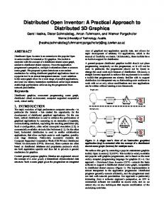
Figure 7: A mesh resulting from subdividing the scene using a SVBSP tree. The darker patches are invisible from the light source. 3.2.6
Global illumination
Beam tracing The beam tracing designed by Heckbert and Hanrahan (1984) casts a pyramid (beam) of rays rather than shooting a single ray at a time. The resulting algorithm makes use of ray coherence and eliminates some aliasing connected with the classical ray tracing.
Cone tracing The cone tracing proposed by Amanatides (1984) traces a cone of rays at a time instead of a polyhedral beam or a single ray. In contrast to the Shadow volumes The shadow volume of a polygon beam tracing the algorithm does not determine precise with respect to a point is a semi infinite frustum. The boundaries of visibility changes. The cones are interintersection of the frustum with the scene bounding sected with the scene objects and at each intersected obvolume can be explicitly reconstructed and represented ject a new cone (or cones) is cast to simulate reflection by a set of shadow polygons bounding the frustum. and refraction. Crow (1977) proposed that these polygons can be used to test if a point corresponding to the pixel of the Bundle tracing Most stochastic global illumination rendered image is in shadow by counting the number methods shoot rays independently and thus they do not of shadow polygons in front of and behind the point. exploit visibility coherence among rays. An excepHeidmann (1991) proposed an efficient real-time im- tion is the ray bundle tracing introduced by Szirmayplementation of the shadow volume algorithm. The Kalos (1998) that shoots a set of parallel rays through shadow volume BSP (SVBSP) tree proposed by Chin the scene according to a randomly sampled direction. and Feiner (1989) provides an efficient representation This approach allows to exploit ray coherence by tracof a union of shadow volumes of a set of convex poly- ing many rays at the same time. gons. The SVBSP tree is used to explicitly compute lit and shadowed fragments of scene polygons. An adapta- 3.2.7 Image-based and Point-based rendering tion of the SVBSP method to dynamic scenes was studied by Chrysanthou and Slater (1995). See Figure 7 for Image-based and point-based rendering generate images from point-sampled representations like images or an illustration of the output of the SVBSP algorithm. 9
point clouds. This is useful for highly complex models, which would otherwise require a huge number of triangles. A point is infinitely small by definition and so the visibility of the point samples is determined using a local reconstruction of the sampled surface that is inherent in the particular rendering algorithm.
line space subdivision maintained by a BSP tree to calculate the PVS. Figure 8 illustrates the concept of a PVS in a 2 12 D scene. 3.3.2
Heidrich et al. (2000) proposed an extension of the shadow map approach for linear light sources (line segments). They use a discrete shadow map enriched by a visibility channel to render soft shadows at interactive speeds. The visibility channel stores the percentage of the light source that is visible at the corresponding point.
Image warping McMillan (1997) proposed an algorithm for warping images from one view point to another. The algorithm resolves visibility by a correct occlusion compatible traversal of the input image without using additional data structures like a z-buffer. Splatting Most point-based rendering algorithms project points on the screen using splatting. Splatting is used to avoid gaps in the image and to resolve visibility of projected points. Pfister et al. (2000) use software visibility splatting. Rusinkiewicz et al. (2000) use a hardware accelerated z-buffer and Grossman and Dally (1998) use the hierarchical z-buffer (Greene et al., 1993) to resolve visibility. Random sampling The randomized z-buffer algorithm proposed by Wand et al. (2001) culls triangles under the assumption that many small triangles project to a single pixel. A large triangle mesh is sampled and visibility of the samples is resolved using the z-buffer. The algorithm selects a sufficient number of sample points so that each pixel receives a sample from a visible triangle with high probability.
3.3
Visibility from a line segment
We discuss visibility from a line segment in the scope of visibility culling and computing soft shadows. 3.3.1
Soft shadows
3.4
Visibility from a polygon
Visibility from a polygon problems are commonly studied by realistic rendering algorithms that aim to capture illumination due to areal light sources. We discuss the following problems: computing soft shadows, evaluating form factors, and discontinuity meshing. 3.4.1 Soft shadows Soft shadows appear in scenes with areal light sources. A shadow due to an areal light source consists of two parts: umbra and penumbra. Umbra is the part of the shadow from which the light source is completely invisible. Penumbra is the part from which the light source is partially visible and partially hidden by some scene objects. The rendering of soft shadows is significantly more difficult than rendering of hard shadows mainly due to complex visibility interactions in penumbra. Ray tracing A straightforward extension of the ray tracing algorithm handles areal light sources by shooting randomly distributed shadow rays towards the light source (Cook et al., 1984).
Visibility culling
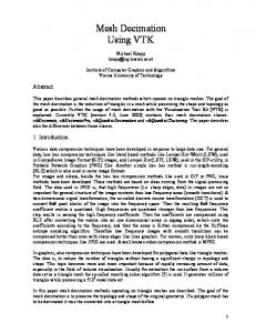
Several algorithms calculate visibility in 2 21 D urban environments for a region of space using a series of visibility from a line segment queries. The PVS for a given view cell is a union of PVSs computed for all ’topedges’ of the viewing region (Wonka et al., 2000). Wonka et al. (2000) use occluder shrinking and point sampling to calculate visibility with the help of a hardware accelerated z-buffer. Koltun et al. (2001) transform the 2 21 D problem to a series of 2D visibility problems. The 2D problems are solved using dual ray space and the z-buffer algorithm. Bittner et al. (2001) use a
Shadow volumes An adaptation of the SVBSP tree for areal light sources was proposed by Chin and Feiner (1992). Chrysanthou and Slater (1997) used a shadow overlap cube to accelerate updates of soft shadows in dynamic polygonal scenes. For each polygon they maintain an approximate discontinuity mesh to accurately capture shadow boundaries (discontinuity meshing will be discussed in the next section). 10
(a)
(b)
(c)
Figure 8: A PVS in a 2 12 D scene representing 8 km2 of Vienna. (a) A selected view cell and the corresponding PVS. The dark regions were culled by hierarchical visibility tests. (b) A closeup of the view cell and its PVS. (c) A snapshot of an observer’s view from a view point inside the view cell. Shadow textures Heckbert and Herf (1997) proposed an algorithm constructing a shadow texture for each scene polygon. The texture is created by smoothed projections of the scene from multiple sample points on the light source. Soler and Sillion (1998) calculate shadow textures using convolution of the ’point-light shadow map’ and an image representing the areal light source.
ray shooting. Campbell and Fussell (1990) extend this method by using a shadow volume BSP tree to resolve visibility.
Discontinuity meshing Discontinuity meshing was introduced by Heckbert (1992) and Lischinski et al. (1992). A discontinuity mesh partitions scene polygons into patches so that each patch ’sees’ a topologi3.4.2 Form-factors cally equivalent view of the light source. Boundaries of Form-factors are used in radiosity (Goral et al., 1984) the mesh correspond to loci of discontinuities in the illuglobal illumination algorithms. A form-factor ex- mination function. The algorithms of Heckbert (1992) presses the mutual transfer of energy between two and Lischinski et al. (1992) construct a subset of the dispatches in the scene. Resolving visibility between the continuity mesh by casting planes corresponding to the patches is crucial for the form-factor computation. vertex-edge visibility events. More elaborated methods capable of creating a complete discontinuity mesh were Hemi-cube The hemi-cube algorithm proposed by introduced by Drettakis and Fiume (1994) and StewCohen and Greenberg (1985) computes a form-factor art and Ghali (1994). Discontinuity meshing can be of a differential area with respect to all patches in the used for computing accurate soft shadows or to anascene. The form-factor between the two patches is es- lytically calculate form-factors with respect to an areal timated by solving visibility at the middle of the patch light source. assuming that the form-factor is almost constant across the patch. Thus the hemi-cube algorithm approximates a visibility from a polygon problem by solving a visi3.5 Visibility from a region bility from a point problem. There are two sources of errors in the hemi-cube algorithm: the finite resolution Visibility from a region problems arise in the context of the hemi-cube and the fact that visibility is sampled of visibility preprocessing. According to our taxonomy only at one point on the patch. the complexity of the from-polygon and from-region visibility in 3D is identical. In fact most visibility from Ray shooting Wallace et al. (1989) proposed a pro- a region algorithms solve the problem by computing a gressive radiosity algorithm that samples visibility by series of from-polygon visibility queries. 11
3.5.1
Visibility culling
of the proposed global visibility algorithms is still an open problem. Prospectively these techniques provide an elegant method for the acceleration of lowerdimensional visibility problems: for example ray shooting can be reduced to a point location in the ray space subdivision.
An offline visibility culling algorithm calculates a PVS of objects that are potentially visible from any point inside a given viewing region. General scenes Durand et al. (2000) proposed extended projections and an occlusion sweep to calculate conservative from-region visibility in general scenes. Schaufler et al. (2000) used blocker extensions to compute conservative visibility in scenes represented as volumetric data. Bittner (2002b) proposed an algorithm using Pl¨ucker coordinates and BSP trees to calculate exact from-region visibility. A similar method was developed by Nirenstein et al. (2002). Indoor scenes Visibility algorithms for indoor scenes exploit the cell/portal subdivision mentioned in Section 3.2.4. Visibility from a cell is computed by checking sequences of portals for possible sight-lines. Airey (1990) used ray shooting to estimate visibility between cells. Teller et al. (1991) and Teller (1992b) use a stabbing line computation to check for feasible portal sequences. Yagel and Ray (1995) present a visibility algorithm for cave-like structures, that uses a regular spatial subdivision.
Visibility complex Pocchiola and Vegter (1993) introduced the visibility complex that describes global visibility in 2D scenes. Rivi`ere (1997) discussed the visibility complex for dynamic polygonal scenes and applied it for maintaining a view around a moving point. The visibility complex was generalized to three dimensions by Durand et al. (1996). No implementation of the 3D visibility complex is known.
Outdoor scenes Outdoor urban scenes are typically considered as of 2 12 D nature and visibility is computed using visibility from a line segment algorithms discussed in Section 3.3.1. Stewart (1997) proposed a conservative hierarchical visibility algorithm that precomputes occluded regions for cells of a digital elevation map. 3.5.2
Aspect graph The aspect graph (Plantinga et al., 1990) partitions the view space into cells that group view points from which the projection of the scene is qualitatively equivalent. The aspect graph is a graph describing the view of the scene (aspect) for each cell of the partitioning. The major drawback of this approach is that for polygonal scenes with n polygons there can be Θ(n9 ) cells in the partitioning for an unrestricted view space.
Sound propagation
Visibility skeleton Durand et al. (1997) introduced the visibility skeleton. The visibility skeleton is a graph describing the skeleton of the 3D visibility complex. The visibility skeleton was implemented and verified experimentally. The results indicate that its worst case complexity O(n4 log n) is much better in practice. Recently Duguet and Drettakis (2002) improved the robustness of the method by using robust epsilonvisibility predicates.
Beam tracing Funkhouser et al. (1998) proposed to use beam-tracing for acoustic modeling in indoor environments. For each cell (region) of the model they construct a beam tree that captures reverberation paths with respect to the cell. The construction of the beam tree is based on the cell/portal visibility algorithms (Airey et al., 1990; Teller & S´equin, 1991).
3.6
Global visibility
Discrete methods Discrete methods describing visibility in a 4D grid-like data structure were proposed by Chrysanthou et al. (1998) and Blais and Poulin (1998). These techniques are closely related to the lumigraph (Gortler et al., 1996) and light field (Levoy & Hanrahan, 1996) used for image-based rendering. Hinkenjann and M¨uller (1996) developed a discrete hierarchical visibility algorithm for 2D scenes. Gotsman et al. (1999) proposed an approximate visibility algorithm that uses a 5D subdivision of ray space and maintains a PVS for each cell of the subdivision. A common problem of discrete global visibility data structures is
The global visibility algorithms typically subdivide lines or rays into equivalence classes according to their visibility classification. A practical application of most 12
their memory consumption required to achieve a reasonable accuracy.
4.1.2
Occluders and occludees
A number of visibility algorithms restructure the scene description to distinguish between occluders and occludees (Zhang et al., 1997; Hudson et al., 1997; Coorg 4 Visibility algorithm design & Teller, 1997; Bittner et al., 1998; Wonka et al., 2000). Occluders are objects that cause changes in visibility In this section we summarize important steps in the de(occlusion). The occluders are used to describe visibilsign of a visibility algorithm and discuss common conity, whereas the occludees are used to check visibility cepts and data structures. Nowadays the research in with respect to the description provided by the occludthe area of visibility is largely driven by the visibility ers. The distinction between occluders and occludees culling methods. This follows from the fact that we are is used mostly by visibility culling algorithms to imconfronted with a large amount of available data that prove the time performance of the algorithm and somecannot be visualized even on the latest graphics hardtimes even its accuracy. Typically, the number of ocware (M¨oller & Haines, 1999). Therefore our discuscluders and occludees is significantly smaller than the sion of the visibility algorithm design is balanced tototal number of objects in the scene. wards efficient concepts introduced recently to solve the Both the occluders and the occludees can be reprevisibility culling problem. sented by ‘virtual’ objects constructed from the scene primitives: the occluders as simplified inscribed objects, occludees as simplified circumscribed objects 4.1 Preparing the data such as bounding boxes. We can classify visibility alWe discuss three issues dealing with the type of data gorithms according to the type of occluders they deal processed by the visibility algorithm: scene restrictions, with. Some algorithms use arbitrary objects as occludidentifying occluders and occludees, and spatial data ers (Greene et al., 1993; Zhang et al., 1997), other algostructures for the scene description. rithms deal only with convex polygons (Hudson et al., 1997; Coorg & Teller, 1997; Bittner et al., 1998), or volumetric cells (Yagel & Ray, 1995; Schaufler et al., 4.1.1 Scene restrictions 2000). Additionally some algorithms require explicit Visibility algorithms can be classified according to the knowledge of occluder connectivity (Coorg & Teller, restrictions they pose on the scene description. The type 1997; Wonka & Schmalstieg, 1999; Schaufler et al., of the scene primitives influences the difficulty of solv- 2000). An important class of occluders are vertical 1 ing the given problem: it is simpler to implement an al- prisms that can be used for computing visibility in 2 2 D gorithm computing a visibility map for scenes consist- scenes (Wonka & Schmalstieg, 1999; Koltun et al., ing of triangles than for scenes with NURBS surfaces. 2001; Bittner et al., 2001) (see Figure 9). As occludees the algorithms typically use bounding The majority of analytic visibility algorithms deals volumes organized in a hierarchical data structure (Woo with static polygonal scenes without transparency. The & Amanatides, 1990; Coorg & Teller, 1997; Wonka polygons are often subdivided into triangles for easier et al., 2000; Koltun et al., 2001; Bittner et al., 2001). manipulation and representation. Some visibility algorithms are designed for volumetric data (Schaufler et al., 2000; Yagel & Ray, 1995), or point clouds (Pfis- 4.1.3 Volumetric scene representation ter et al., 2000). Analytic handling of parametric, implicit or procedural objects is complicated and so these The scene is typically represented by a collection of objects are typically converted to a boundary represen- objects. For purposes of visibility computations it can tation. be advantageous to transform the object centered repreMany discrete algorithms can handle complicated sentation to a volumetric representation (Yagel & Ray, objects by sampling their surface (e.g. the z-buffer, ray 1995; Saona-V´azquez et al., 1999; Schaufler et al., casting). In particular the ray shooting algorithm (Ap- 2000). For example the scene can be represented by pel, 1968) solving visibility along a single line can di- an octree where full voxels correspond to opaque parts rectly handle CSG models, parametric and implicit sur- of the scene. This representation provides a regular description of the scene that avoids complicated configufaces, subdivision surfaces, etc. 13
algorithm solves visibility using a transformation of the problem to line space or ray space. Image space algorithms can also be seen as an important subclass of line space methods for computing visibility from a point problems in 3D. The image space methods solve visibility in a plane that represents the problem-relevant line set L3p : each ray originating at the given point corresponds to a point in the image plane. Note that in our classification even an image space algorithm can be continuous and an object space algorithm can be discrete. This classification differs from the understanding of image space and object space algorithms that considers all image space algorithms discrete and all object space algorithms continuous (Sutherland et al., 1974).
Figure 9: Occluders in an urban scene. In urban scenes the occluders can be considered vertical prisms erected above the ground.
4.3
According to the accuracy of the result visibility algorithms can be classified into the following three categories (Cohen-Or et al., 2002):
rations or overly detailed input. Furthermore, the representation is independent of the total scene complexity.
4.2
Accuracy
• exact,
The core: solution space data structures
• conservative, • approximate.
The solution space is the domain in which the algorithm determines the desired result. For most visibility algorithms the solution space data structure represents the invisible (occluded) volume or its boundaries. In the case that the dimension of the solution space matches the dimension of the problem-relevant line set, the visibility problem can often be solved with high accuracy by a single sweep through the scene (Bittner, 2002b). Visibility algorithms can be classified according to the structure of the solution space as discrete or continuous. For example the z-buffer (Catmull, 1975) is a common example of a discrete algorithm whereas the Weiler-Atherton algorithm (Weiler & Atherton, 1977) is an example of a continuous one. We can further distinguish the algorithms according to the semantics of the solution space (a similar classification was given by Durand (1999)):
An exact algorithm provides an exact analytic result for the given problem (in practice however this result is commonly influenced by the finite precision of the floating point arithmetics). A conservative algorithm overestimates visibility, i.e. it never misses any visible object, surface or point. An approximate algorithm provides only an approximation of the result, i.e. it can both overestimate and underestimate visibility. The classification according to the accuracy can be illustrated easily on computing a PVS: an exact algorithm computes an exact PVS. A conservative algorithm computes a superset of the exact PVS. An approximate algorithm computes an approximation to the exact PVS that is neither its subset nor its superset considering all possible inputs. A more precise measure of the accuracy can be expressed as a distance from an exact result in the solution space. For example, in the case of PVS algorithms we could evaluate relative overestimation and relative underestimation of the PVS with respect to the exact PVS. In the case of discontinuity meshing we can classify algorithms according to the classes of visibility events they deal with (Stewart & Ghali, 1994; Durand, 1999).
• primal space (object space) • dual space (image space, line space, ray space) A primal space algorithm solves the problem by studying the visibility between objects without a transformation to a different solution space. A dual space 14
In the next section we discuss an intuitive classification of the ability of a visibility algorithm to capture occlusion. 4.3.1
Sutherland et al. (1974) identified several different types of coherence in the context of visible surface algorithms. We simplify the classification proposed by Sutherland to reflect general visibility algorithms and distinguish between the following three types of visibility coherence:
Occluder fusion
The occluder fusion is the ability of a visibility algorithm to account for the combined effect of multiple occluders. We can distinguish three types of fusion of umbra for visibility from a point algorithms. In the case of visibility from a region there are additional four types that express fusion of penumbra (see Figure 10).
4.4
• Spatial coherence. Visibility of points in space tends to be coherent in the sense that the visible part of the scene consists of compact sets (regions) of visible and invisible points.
Achieving performance
• Image-space, line-space, or ray-space coherence. Sets of similar rays tend to have the same visibility classification, i.e. the rays intersect the same object.
This section discusses four issues related to the running time and the memory consumption: scalability, acceleration data structures, and the use of graphics hardware. 4.4.1
• Temporal coherence. Visibility at two successive moments is likely to be similar despite small changes in the scene or a region/point of interest. The degree to which an algorithm exploits various types of coherence is one of the major design paradigms in research of new visibility algorithms. The importance of exploiting coherence is emphasized by the large amount of data that need to be processed by the current rendering algorithms.
Scalability
Scalability expresses the ability of the visibility algorithm to cope with larger inputs. The scalability of an algorithm can be studied with respect to the size of the scene (e.g. number of scene objects). Another measure might consider the dependence of the algorithm on the number of the visible objects. Scalability can also be studied according to the given domain restrictions, e.g. volume of the view cell. A well designed visibility algorithm should be scalable with respect to the number of structural changes of visibility. Furthermore, its performance should be given by the complexity of the visible part of the scene. These two important measures of scalability of an algorithm are discussed in the next two sections.
Output sensitivity An algorithm is said to be output sensitive if its running time is sensitive to the size of output (Gotsman et al., 1999). In the computer graphics community the term output sensitive algorithm is used in a broader meaning than in computational geometry (Berg et al., 1997). The attention is paid to a practical usage of the algorithm, i.e. to an efficient implementation in terms of the practical average case performance. The algorithms are usually evaluated experimentally using several data sets and measuring the running time and the size of output of the algorithm.
Use of coherence Scenes in computer graphics typically consist of objects whose properties vary smoothly. A view of such a scene contains regions of smooth changes (changes in color, depth, texture,etc.) at the surface of one object and discontinuities between objects. The degree to which the scene or its projection exhibit local similarities is called coherence (Foley et al., 1990). Coherence can be exploited by reusing calculations made for one part of the scene for nearby parts. Algorithms exploiting coherence are typically more efficient than algorithms computing the result from the scratch.
4.4.2
Visibility preprocessing
15
Visibility computations at runtime can be accelerated by visibility preprocessing. The time for preprocessing is often amortized over many executions of runtime visibility queries (M¨oller & Haines, 1999). A typical application where visibility preprocessing is used are walkthroughs of complex geometric models (Airey et al., 1990). In this case visibility is preprocessed by finding a PVS for all view cells in the scene. At run-time only the PVS corresponding to the location of the view point
object, classified visible object, classified invisible viewpoint view cell calculated occlusion
viewpoint a) no fusion
b) connected occluder fusion
c) complete fusion
view cell
d) no fusion
e) connected occluder fusion f) overlapping umbra fusion g) complete fusion
Figure 10: Illustration of occluder fusion. Occluders are shown as black lines and occludees as circles. An occludee that is marked white is classified visible due to the lack of occluder fusion. is considered for rendering. The drawbacks of visibility preprocessing are the memory consumption of the precomputed visibility information and a complicated handling of dynamic changes.
such as the pixel and vertex shaders allow easier application of the graphics hardware for solving specific visibility tasks (Purcell et al., 2002).
4.5 4.4.3
Acceleration data structures
4.4.4
Use of graphics hardware
Visibility algorithm template
We provide a general outline of an output sensitive visAcceleration data structures are used to achieve the ibility algorithm for calculating visibility from a point performance goals of a visibility algorithm (M¨oller & or a region. In a preprocessing step occluders and ocHaines, 1999; Havran, 2000). These data structures cludees are constructed and the scene is organized in a allow efficient point location, proximity queries, or spatial data structure (e.g. kD-tree). To calculate visiscene traversal required by many visibility algorithms. bility for a view point or a region we need a data strucThe common acceleration data structures include spa- ture describing the occlusion with respect to the point tial subdivisions and bounding volume hierarchies that or the region. The algorithm proceeds as follows: group scene objects according to the spatial proximity. • The kD-tree is traversed top-down and front to Another class of acceleration data structures consists of back. data structures that group rays according to their prox• For each kD-tree node test the node against the ocimity in dual space (line space or ray space). clusion data structure. • If the node is invisible cull its subtree and proceed with the next node.
The hardware implementation of the z-buffer algorithm is available even on a low-end graphics hardware. The hardware z-buffer can be used to accelerate solutions to other visibility problems. A visibility algorithm can be accelerated by the graphics hardware if it can be decomposed into a series of z-buffer steps. Recall that the zbuffer algorithm solves the visibility from a point problem by providing a discrete approximation of the visible surfaces. The recent features of the graphics hardware,
• If the node is visible and it is not a leaf, descend into its subtree. • If the node is visible and it is leaf: (1) Insert the occluders in the node to the occlusion data structure. (2) Mark all occludees associated with the node as visible.
16
onomy that aims to classify visibility problems independently of their target application. The classification should help to understand the nature of the given problem and it should assist in finding relationships between visibility problems and algorithms in different application areas. We aimed to provide a representative sample of visibility algorithms for visible surface determination, visibility culling, shadow computation, image-based and point-based rendering, global illumination, and global visibility computations. We discussed common concepts of visibility algorithm design that should help to assist an algorithm designer to transfer existing algorithms for solving visibility problems. Finally, we summarized visibility algorithms discussed in the paper according to their domain, solution space, and accuracy. Computer graphics offers a number of efficient visibility algorithms for all stated visibility problems in 2D as well as visibility along a line and visibility from a point in 3D. In particular it provides a well researched background for discrete techniques. The solution of higher dimensional visibility is significantly more difficult. The discrete techniques require a large number of samples to achieve satisfying accuracy, whereas the continuous techniques are prone to robustness problems and are difficult to implement. The existing solutions must be tuned to a specific application. Therefore the problems of visibility from a line segment, a polygon, a region, and global visibility problems in 3D are the main focus of active computer graphics research in visibility.
Many efficient visibility culling algorithms follow this outline (Greene et al., 1993; Bittner et al., 1998; Wonka & Schmalstieg, 1999; Downs et al., 2001; Bittner et al., 2001; Wonka et al., 2000). Graphics hardware can be used to accelerate the updates of the occlusion data structure. On the other hand the occlusion test becomes more complicated because of hardware restrictions (Wonka & Schmalstieg, 1999; Durand et al., 2000; Zhang et al., 1997).
4.6
Summary
In this section we discussed common concepts of visibility algorithm design and mentioned several criteria used for the classification of visibility algorithms. Although the discussion was balanced towards visibility culling methods we believe that it provides a useful overview even for other visibility problems. To sum up the algorithms discussed in the paper we provide two overview tables. Table 2 reviews algorithms for visibility from a point, Table 3 reviews algorithms for visibility from a line segment, a polygon, a region, and global visibility. The algorithms are indexed according to the problem domain, the actual visibility problem, and the structure of the domain. We characterize each algorithm using three features: solution space structure, solution space semantics, and accuracy. These features were selected as they provide a meaningful classification for the broad class of algorithms discussed in the paper. The solution space semantics is classified as follows: If the algorithm solves visibility in an image plane we classify it as image space. Note, that this plane does not need to correspond to the viewing plane (e.g. shadow map). Similarly, if the algorithm solves visibility using line space or ray space analogies, we classify it as line space or ray space, respectively. If the algorithm solves visibility using object space entities (e.g. shadow volume boundaries), we classify it as object space. The accuracy is expressed with respect to the problem domain structure. This means that if the algorithm solves a problem with a discrete domain it can still provide an exact result although it evaluates visibility only for the discrete samples.
Acknowledgments This research was supported by the Czech Ministry of Education under Project LN00B096 and the Austrian Science Foundation (FWF) contract no. p-13876-INF.
5 Conclusion Visibility problems and algorithms penetrate a large part of computer graphics research. We proposed a tax17
domain
problem description
domain structure
solution space structure semantics
algorithm
Catmull (1975) Newell et al. (1972) Fuchs et al. (1980) visible D Gordon & Chen (1991) surface Warnock (1969) determination Appel (1968) Naylor (1992) C Weiler & Atherton (1977) Greene et al. (1993) Zhang et al. (1997) Aila (2000) D Hey et al. (2001) Klosowski & Silva. (2001) Cohen-Or & Shaked (1995) visibility Lee & Shin (1997) culling Luebke & Georges (1995) Coorg & Teller (1997) Hudson et al. (1997) C Bittner et al. (1998) Wonka & Schmalstieg (1999) VFP Downs et al. (2001) Lloyd & Egbert (2002) visibility Stewart & Karkanis (1998) C maps Bittner (2002a) Whitted (1979) Haines & Greenberg (1986) Woo & Amanatides (1990) Williams (1978) D hard Segal et al. (1992) shadows Stamminger & Drettakis (2002) Crow (1977) Heidmann (1991) Chin & Feiner (1989) C Chrysanthou & Slater (1995) Heckbert & Hanrahan (1984) ray-set C Amanatides (1984) tracing Szirmay-Kalos & Purgathofer (1998) McMillan (1997) Pfister et al. (2000) point-based D Rusinkiewicz & Levoy (2000) rendering Grossman & Dally (1998) Wand et al. (2001) Problem domain structure: D - discrete, C - continuous.
D C/D C/D C/D D D C C D D D D D D D C C C C D C C D C D D D D D D C/D C/D C C C C D D D D D D
accuracy
I O/I O/I O/I I O O/I I I I I I I O O I O O O O I I I O/I O I O I I I O O O O I O I I I I I I
Solution space structure: D - discrete, C - continuous. Solution space semantics: O - object space, I - image space. Accuracy: E - exact, C - conservative, A - approximate.
Table 2: Summary of visibility from a point algorithms.
18
E E E E E E E E C C/A C/A C C E E C C C C C C C A E E C C A A A E E E E E A A E A A A A
notes HW
HW HW HW HW terrains terrains indoor
HW 2 12 D terrains HW
HW HW HW dynamic
HW
HW HW HW
domain
problem description
solution space structure semantics
algorithm
Heidrich et al. (2000) Wonka et al. (2000) C Koltun et al. (2001) Bittner et al. (2001) D Cook et al. (1984) soft shadows Chin & Feiner (1992) Chrysanthou & Slater (1997) C Heckbert & Herf (1997) Soler & Sillion (1998) Cohen & Greenberg (1985) VFPo form-factors C Wallace et al. (1989) Campbell, III & Fussell (1990) Heckbert (1992) discontinuity Lischinski et al. (1992) C meshing Drettakis & Fiume (1994) Stewart & Ghali (1994) Durand et al. (2000) Schaufler et al. (2000) Bittner (2002b) Nirenstein et al. (2002) visibility VFR C Airey et al. (1990) culling Teller & S´equin (1991) Teller (1992b) Yagel & Ray (1995) Stewart (1997) aspect graph C Plantinga et al. (1990) Pocchiola & Vegter (1993) Rivi`ere (1997) visibility C Durand et al. (1996) complex Durand et al. (1997) GV Duguet & Drettakis (2002) Hinkenjann & M¨uller (1996) discrete Blais & Poulin (1998) C structures Chrysanthou et al. (1998) Gotsman et al. (1999) Problem domain structure: D - discrete, C - continuous. Solution space structure: D - discrete, C - continuous. Solution space semantics: O - object space, L - line space, R - ray space. Accuracy: E - exact, C - conservative, A - approximate. VLS
soft shadows visibility culling in 2 12 D
domain structure D
D D D C D C C D D D D C C C C C D D C C D C C D C C C C C C C D D D D
I O O/L L/O O O O I/O I/O I O O O O O O I/O O L L O L L O O O L L L O O L L R R
accuracy A C C C A A A A A A A A A A E E C C E E A E E C C E E E E E E/A A A A A
notes HW HW
dynamic HW HW HW
HW
indoor indoor 2D indoor caves terrain 2D 2D
2D
Table 3: Summary of algorithms for visibility from a line segment, visibility from a polygon, visibility from a region, and global visibility.
19
References
Catmull, E.E. (1975). Computer display of curved surfaces. In Proceedings of the IEEE Conference on Computer Graphics, Pattern Recognition, and Data Structure, 11–17.
Aila, T. (2000). SurRender Umbra: A Visibility Determination Framework for Dynamic Environments. Master’s thesis, Helsinki University of Technology. Airey, J.M., Rohlf, J.H. & Brooks, Jr., F.P. (1990). Towards image realism with interactive update rates in complex virtual building environments. In 1990 Symposium on Interactive 3D Graphics, 41–50, ACM SIGGRAPH. Amanatides, J. (1984). Ray tracing with cones. In Computer Graphics (SIGGRAPH ’84 Proceedings), vol. 18, 129–135. Appel, A. (1968). Some techniques for shading machine renderings of solids. In AFIPS 1968 Spring Joint Computer Conf., vol. 32, 37–45. Arvo, J. & Kirk, D. (1989). A survey of ray tracing acceleration techniques, 201–262. Academic Press. Arvo, J. & Kirk, D. (1990). Particle transport and image synthesis. In F. Baskett, ed., Computer Graphics (Proceedings of SIGGRAPH’90), 63–66. Berg, M., Kreveld, M., Overmars, M. & Schwarzkopf, O. (1997). Computational Geometry: Algorithms and Applications. Springer-Verlag, Berlin, Heidelberg, New York. Bittner, J. (2002a). Efficient construction of visibility maps using approximate occlusion sweep. In Proceedings of Spring Conference on Computer Graphics (SCCG’02), 163–171, Budmerice, Slovakia. Bittner, J. (2002b). Hierarchical Techniques for Visibility Computations. Ph.D. thesis, Czech Technical University in Prague. Bittner, J., Havran, V. & Slav´ık, P. (1998). Hierarchical visibility culling with occlusion trees. In Proceedings of Computer Graphics International ’98 (CGI’98), 207–219, IEEE.
Chin, N. & Feiner, S. (1989). Near real-time shadow generation using BSP trees. In Computer Graphics (Proceedings of SIGGRAPH ’89), 99–106. Chin, N. & Feiner, S. (1992). Fast object-precision shadow generation for areal light sources using BSP trees. In D. Zeltzer, ed., Computer Graphics (1992 Symposium on Interactive 3D Graphics), vol. 25, 21–30. Chrysanthou, Y. & Slater, M. (1995). Shadow volume BSP trees for computation of shadows in dynamic scenes. In P. Hanrahan & J. Winget, eds., 1995 Symposium on Interactive 3D Graphics, 45–50, ACM SIGGRAPH, iSBN 0-89791-736-7. Chrysanthou, Y. & Slater, M. (1997). Incremental updates to scenes illuminated by area light sources. In Proceedings of Eurographics Workshop on Rendering, 103–114, Springer Verlag. Chrysanthou, Y., Cohen-Or, D. & Lischinski, D. (1998). Fast approximate quantitative visibility for complex scenes. In Proceedings of Computer Graphics International ’98 (CGI’98), 23–31, IEEE, NY, Hannover, Germany. Cohen, M.F. & Greenberg, D.P. (1985). The hemi-cube: A radiosity solution for complex environments. Computer Graphics (SIGGRAPH ’85 Proceedings), 19, 31–40. Cohen-Or, D. & Shaked, A. (1995). Visibility and dead-zones in digital terrain maps. Computer Graphics Forum, 14, C/171–C/180. Cohen-Or, D., Chrysanthou, Y., Silva, C. & Durand, F. (2002). A survey of visibility for walkthrough applications. To appear in IEEE Transactions on Visualization and Computer Graphics..
Bittner, J., Wonka, P. & Wimmer, M. (2001). Visibility preprocessing for urban scenes using line space subdivision. In Proceedings of Pacific Graphics (PG’01), 276–284, IEEE Computer Society, Tokyo, Japan.
Cook, R.L., Porter, T. & Carpenter, L. (1984). Distributed ray tracing. In Computer Graphics (SIGGRAPH ’84 Proceedings), 137–45.
Blais, M. & Poulin, P. (1998). Sampling visibility in threespace. In Proc. of the 1998 Western Computer Graphics Symposium, 45–52.
Coorg, S. & Teller, S. (1997). Real-time occlusion culling for models with large occluders. In Proceedings of the Symposium on Interactive 3D Graphics, 83–90, ACM Press, New York.
Campbell, III, A.T. & Fussell, D.S. (1990). Adaptive mesh generation for global diffuse illumination. In Computer Graphics (SIGGRAPH ’90 Proceedings), vol. 24, 155–164.
Crow, F.C. (1977). Shadow algorithms for computer graphics. Computer Graphics (SIGGRAPH ’77 Proceedings), 11.
Carpenter, L. (1984). The A-buffer, an antialiased hidden surface method. In H. Christiansen, ed., Computer Graphics (SIGGRAPH ’84 Proceedings), vol. 18, 103–108.
Downs, L., M¨oller, T. & S´equin, C.H. (2001). Occlusion horizons for driving through urban scenes. In Symposium on Interactive 3D Graphics, 121–124, ACM SIGGRAPH.
20
Drettakis, G. & Fiume, E. (1994). A Fast Shadow Algorithm for Area Light Sources Using Backprojection. In Computer Graphics (Proceedings of SIGGRAPH ’94), 223–230.
Gotsman, C., Sudarsky, O. & Fayman, J.A. (1999). Optimized occlusion culling using five-dimensional subdivision. Computers and Graphics, 23, 645–654.
Duguet, F. & Drettakis, G. (2002). Robust epsilon visibility. Computer Graphics (SIGGRAPH’02 Proceedings).
Grant, C.W. (1992). Visibility Algorithms in Image Synthesis. Ph.D. thesis, U. of California, Davis.
Durand, F. (1999). 3D Visibility: Analytical Study and Applications. Ph.D. thesis, Universite Joseph Fourier, Grenoble, France.
Grasset, J., Terraz, O., Hasenfratz, J.M. & Plemenos, D. (1999). Accurate scene display by using visibility maps. In Spring Conference on Computer Graphics and its Applications.
Durand, F., Drettakis, G. & Puech, C. (1996). The 3D visibility complex: A new approach to the problems of accurate visibility. In Proceedings of Eurographics Rendering Workshop ’96, 245–256, Springer.
Greene, N., Kass, M. & Miller, G. (1993). Hierarchical Zbuffer visibility. In Computer Graphics (Proceedings of SIGGRAPH ’93), 231–238. Grossman, J.P. & Dally, W.J. (1998). Point sample rendering. In Rendering Techniques ’98 (Proceedings of Eurographics Rendering Workshop), 181–192, Springer-Verlag Wien New York.
Durand, F., Drettakis, G. & Puech, C. (1997). The visibility skeleton: A powerful and efficient multi-purpose global visibility tool. In Computer Graphics (Proceedings of SIGGRAPH ’97), 89–100. Durand, F., Drettakis, G., Thollot, J. & Puech, C. (2000). Conservative visibility preprocessing using extended projections. In Computer Graphics (Proceedings of SIGGRAPH 2000), 239–248.
Gu, X., Gortier, S.J. & Cohen, M.F. (1997). Polyhedral geometry and the two-plane parameterization. In J. Dorsey & P. Slusallek, eds., Eurographics Rendering Workshop 1997, 1–12, Eurographics, Springer Wein, New York City, NY, iSBN 3-211-83001-4.
Floriani, L.D. & Magillo, P. (1995). Horizon computation on a hierarchical terrain model. The Visual Computer: An International Journal of Computer Graphics, 11, 134–149.
Haines, E.A. & Greenberg, D.P. (1986). The light buffer: A ray tracer shadow testing accelerator. IEEE Computer Graphics and Applications, 6, 6–16.
Foley, J.D., van Dam, A., Feiner, S.K. & Hughes, J.F. (1990). Computer Graphics: Principles and Practice. AddisonWesley Publishing Co., Reading, MA, 2nd edn.
Havran, V. (2000). Heuristic Ray Shooting Algorithms. Ph.d. thesis, Department of Computer Science and Engineering, Faculty of Electrical Engineering, Czech Technical University in Prague.
Fuchs, H., Kedem, Z.M. & Naylor, B.F. (1980). On visible surface generation by a priori tree structures. In Computer Graphics (SIGGRAPH ’80 Proceedings), vol. 14, 124–133. Funkhouser, T., Carlbom, I., Elko, G., Pingali, G., Sondhi, M. & West, J. (1998). A beam tracing approach to acoustic modeling for interactive virtual environments. In Computer Graphics (Proceedings of SIGGRAPH ’98), 21–32.
Heckbert, P.S. (1992). Discontinuity meshing for radiosity. In Third Eurographics Workshop on Rendering, 203–216, Bristol, UK. Heckbert, P.S. & Hanrahan, P. (1984). Beam tracing polygonal objects. Computer Graphics (SIGGRAPH’84 Proceedings), 18, 119–127. Heckbert, P.S. & Herf, M. (1997). Simulating soft shadows with graphics hardware. Tech. rep., CS Dept., Carnegie Mellon U., cMU-CS-97-104, http://www.cs.cmu.edu/ ph.
Goral, C.M., Torrance, K.K., Greenberg, D.P. & Battaile, B. (1984). Modelling the interaction of light between diffuse surfaces. In Computer Graphics (SIGGRAPH ’84 Proceedings), vol. 18, 213–222. Gordon, D. & Chen, S. (1991). Front-to-back display of BSP trees. IEEE Computer Graphics and Applications, 11, 79– 85.
Heidmann, T. (1991). Real shadows, real time. Iris Universe, 18, 28–31, silicon Graphics, Inc.
Gortler, S.J., Grzeszczuk, R., Szeliski, R. & Cohen, M.F. (1996). The lumigraph. In Computer Graphics (SIGGRAPH ’96 Proceedings), Annual Conference Series, 43– 54, Addison Wesley.
Heidrich, W., Brabec, S. & Seidel, H. (2000). Soft shadow maps for linear lights. In Proceedings of EUROGRAPHICS Workshop on Rendering, 269–280.
21
Hey, H., Tobler, R.F. & Purgathofer, W. (2001). Real-Time occlusion culling with a lazy occlusion grid. In Proceedings of EUROGRAPHICS Workshop on Rendering, 217–222.
Hinkenjann, A. & M¨uller, H. (1996). Hierarchical blocker trees for global visibility calculation. Research Report 621/1996, University of Dortmund.
Newell, M.E., Newell, R.G. & Sancha, T.L. (1972). A solution to the hidden surface problem. In Proceedings of ACM National Conference.
Hudson, T., Manocha, D., J.Cohen, M.Lin, K.Hoff & H.Zhang (1997). Accelerated occlusion culling using shadow frusta. In Proceedings of the Thirteenth ACM Symposium on Computational Geometry, June 1997, Nice, France.
Nirenstein, S., Blake, E. & Gain, J. (2002). Exact FromRegion visibility culling. In Proceedings of EUROGRAPHICS Workshop on Rendering, 199–210.
Kajiya, J.T. (1986). The rendering equation. In Computer Graphics (SIGGRAPH ’86 Proceedings), 143–150.
Pellegrini, M. (1997). Ray shooting and lines in space. In J.E. Goodman & J. O’Rourke, eds., Handbook of Discrete and Computational Geometry, chap. 32, 599–614, CRC Press LLC, Boca Raton, FL.
Klosowski, J.T. & Silva., C.T. (2001). Efficient conservative visibility culling using the prioritized-layered projection algorithm. IEEE Transactions on Visualization and Computer Graphics, 7, 365–379.
Pfister, H., Zwicker, M., van Baar, J. & Gross, M. (2000). Surfels: Surface elements as rendering primitives. In Computer Graphics (Proceedings of SIGGRAPH 2001), 335– 342, ACM SIGGRAPH / Addison Wesley Longman.
Koltun, V., Chrysanthou, Y. & Cohen-Or, D. (2001). Hardware-accelerated from-region visibility using a dual ray space. In Proceedings of the 12th EUROGRAPHICS Workshop on Rendering.
Plantinga, H., Dyer, C.R. & Seales, W.B. (1990). Real-time hidden-line elimination for a rotating polyhedral scene using the aspect representation. In Proceedings of Graphics Interface ’90, 9–16.
Lee, C.H. & Shin, Y.G. (1997). A terrain rendering method using vertical ray coherence. The Journal of Visualization and Computer Animation, 8, 97–114.
Pocchiola, M. & Vegter, G. (1993). The visibility complex. In Proc. 9th Annu. ACM Sympos. Comput. Geom., 328–337.
Levoy, M. & Hanrahan, P. (1996). Light field rendering. In H. Rushmeier, ed., SIGGRAPH 96 Conference Proceedings, Annual Conference Series, 31–42, ACM SIGGRAPH, Addison Wesley, held in New Orleans, Louisiana, 04-09 August 1996. Lischinski, D., Tampieri, F. & Greenberg, D.P. (1992). Discontinuity meshing for accurate radiosity. IEEE Computer Graphics and Applications, 12, 25–39. Lloyd, B. & Egbert, P. (2002). Horizon occlusion culling for real-time rendering of hierarchical terrains. In Proceedings of the conference on Visualization ’02, 403–410, IEEE Press. Luebke, D. & Georges, C. (1995). Portals and mirrors: Simple, fast evaluation of potentially visible sets. In P. Hanrahan & J. Winget, eds., 1995 Symposium on Interactive 3D Graphics, 105–106, ACM SIGGRAPH. McMillan, L. (1997). An image-based approach to threedimensional computer graphics. Ph.D. Thesis TR97-013, University of North Carolina, Chapel Hill.
Purcell, T.J., Buck, I., Mark, W.R. & Hanrahan, P. (2002). Ray tracing on programmable graphics hardware. In Computer Graphics (SIGGRAPH ’02 Proceedings), 703–712. Rivi`ere, S. (1997). Dynamic visibility in polygonal scenes with the visibility complex. In Proc. 13th Annu. ACM Sympos. Comput. Geom., 421–423. Rusinkiewicz, S. & Levoy, M. (2000). QSplat: A multiresolution point rendering system for large meshes. In Computer Graphics (Proceedings of SIGGRAPH 2000), 343– 352, ACM SIGGRAPH / Addison Wesley Longman. Saona-V´azquez, C., Navazo, I. & Brunet, P. (1999). The visibility octree: a data structure for 3D navigation. Computers and Graphics, 23, 635–643. Schaufler, G., Dorsey, J., Decoret, X. & Sillion, F.X. (2000). Conservative volumetric visibility with occluder fusion. In Computer Graphics (Proceedings of SIGGRAPH 2000), 229–238.
M¨oller, T. & Haines, E. (1999). Real-Time Rendering. A. K. Peters Limited.
Segal, M., Korobkin, C., van Widenfelt, R., Foran, J. & Haeberli, P. (1992). Fast shadows and lighting effects using texture mapping. Computer Graphics (SIGGRAPH ’92 Proceedings), 26, 249–252.
Naylor, B.F. (1992). Partitioning tree image representation and generation from 3D geometric models. In Proceedings of Graphics Interface ’92, 201–212.
Soler, C. & Sillion, F. (1998). Fast calculation of soft shadow textures using convolution. In Computer Graphics (Proceedings of SIGGRAPH ’98), ACM SIGGRAPH.
22
Warnock, J. (1969). A hidden-surface algorithm for computer generated half-tone pictures. Tech. Rep. TR 4–15, NTIS AD-733 671, University of Utah, Computer Science Department.
Stamminger, M. & Drettakis, G. (2002). Perspective shadow maps. In SIGGRAPH 2002 Conference Proceedings, 557– 562, ACM Press/ ACM SIGGRAPH. Stewart, A.J. (1997). Hierarchical visibility in terrains. In Proceedings of Eurographics Rendering Workshop ’97, 217– 228. Stewart, A.J. & Ghali, S. (1994). Fast computation of shadow boundaries using spatial coherence and backprojections. In Computer Graphics (Proceedings of SIGGRAPH ’94), 231–238. Stewart, A.J. & Karkanis, T. (1998). Computing the approximate visibility map, with applications to form factors and discontinuity meshing. In Proceedings of the Ninth Eurographics Workshop on Rendering, 57–68. Stolfi, J. (1991). Oriented Projective Geometry: A Framework for Geometric Computations. Academic Press. Sutherland, I.E., Sproull, R.F. & Schumacker, R.A. (1974). A characterization of ten hidden-surface algorithms. ACM Computing Surveys, 6, 1–55. Szirmay-Kalos, L. & Purgathofer, W. (1998). Global raybundle tracing with hardware acceleration. In Ninth Eurographics Workshop on Rendering, Vienna, Austria. Teller, S.J. (1992a). Computing the antipenumbra of an area light source. In Computer Graphics (Proceedings of SIGGRAPH ’92), 139–148. Teller, S.J. (1992b). Visibility Computations in Densely Occluded Polyhedral Environments. Ph.D. thesis, CS Division, UC Berkeley, tech. Report UCB/CSD-92-708. Teller, S.J. & S´equin, C.H. (1991). Visibility preprocessing for interactive walkthroughs. In Proceedings of SIGGRAPH ’91, 61–69. Wald, I., Slusallek, P., Benthin, C. & Wagner, M. (2001). Interactive rendering with coherent ray tracing. In A. Chalmers & T.M. Rhyne, eds., EG 2001 Proceedings, vol. 20(3) of Computer Graphics Forum, 153–164, Blackwell Publishing.
Weiler, K. & Atherton, P. (1977). Hidden surface removal using polygon area sorting. In Computer Graphics (SIGGRAPH ’77 Proceedings), 214–222. Whitted, T. (1979). An improved illumination model for shaded display. In Computer Graphics (Special SIGGRAPH ’79 Issue), vol. 13, 1–14. Williams, L. (1978). Casting curved shadows on curved surfaces. In Computer Graphics (SIGGRAPH ’78 Proceedings), 270–274. Wonka, P. & Schmalstieg, D. (1999). Occluder shadows for fast walkthroughs of urban environments. In Computer Graphics Forum (Proceedings of EUROGRAPHICS ’99), 51–60, Blackwell Publishers. Wonka, P., Wimmer, M. & Schmalstieg, D. (2000). Visibility preprocessing with occluder fusion for urban walkthroughs. In Proceedings of EUROGRAPHICS Workshop on Rendering, 71–82. Woo, A. & Amanatides, J. (1990). Voxel occlusion testing: A shadow determination accelerator for ray tracing. In Proceedings of Graphics Interface ’90, 213–220. Woo, A., Poulin, P. & Fournier, A. (1990). A survey of shadow algorithms. IEEE Computer Graphics and Applications, 10, 13–32. Yagel, R. & Ray, W. (1995). Visibility computation for efficient walkthrough of complex environments. Presence: Teleoperators and Virtual Environments, 5. Zhang, H., Manocha, D., Hudson, T. & Hoff III, K.E. (1997). Visibility culling using hierarchical occlusion maps. In Computer Graphics (Proceedings of SIGGRAPH ’97), 77– 88.
Wallace, J.R., Elmquist, K.A. & Haines, E.A. (1989). A ray tracing algorithm for progressive radiosity. In SIGGRAPH ’89 Proceedings, 315–324. Wand, M., Fischer, M., Peter, I., auf der Heide, F.M. & Straßer, W. (2001). The randomized z-buffer algorithm: Interactive rendering of highly complex scenes. In Computer Graphics (Proceedings of SIGGRAPH 2001), 361– 370, ACM SIGGRAPH.
23