For NGI 2008
Method of DiffServ-Based Bandwidth-Sharing among Delay-Sensitive Traffic and Loss-Sensitive Traffic in Backbones Yasusi Kanada Central Research Laboratory, Hitachi, Ltd. Higashi-Koigakubo 1-280, Kokubunji, Tokyo 185-8601, Japan
[email protected] Abstract: Real-time and multimedia applications require an end-to-end QoS guarantee, and various types of applications require various QoS conditions. A DiffServ network should guarantee different QoS conditions for different types of communications. In this paper, the effect of traffic control in a DiffServ core network is experimentally evaluated using bursty traffic generated by an MMPP (Markov-Modulated Poisson Process) model. The situation to be simulated is that there are hundreds of conversational video streams that are delay-sensitive and hundreds of streaming videos that are loss-sensitive. If there are bandwidth-sharing queues such as those follow WFQ (Weighted Fair Queuing) in the core nodes and the two types of video traffic are assigned to two of the queues, the requirements of both types of traffic can be satisfied in a better (more efficient) way by assigning a larger weight to the queue for the conversational video. In our experiment using MMPP-based actual traffic and highend L3 switches, the optimum ratio of the weights was approximately 1.3 when the traffic rates were the same. The optimum weight shares depend on the nature of the traffic, especially the burstiness. Keywords: NGN, Next-generation backbone, QoS measurement, QoS guarantee, DiffServ, Bandwidth sharing, WFQ.
should be different from quantity-oriented communication services because the QoS requirements are more quality oriented, i.e., measured by multi-dimensional parameters such as latency, jitter, and loss ratio for example. A DiffServ network should and can guarantee different QoS conditions for different types of communications, and probably, the network resources can be used more efficiently by a method of quality-oriented QoS guarantee. In this paper, the author intends to show a method of quality-oriented QoS guarantee and an example of a multiservice core network with a quality-oriented QoS guarantee by experiments using actual network nodes and computergenerated network traffic instead of a mere computer simulation or theory. We generated and used two types of traffic that simulate conversational and streaming video traffic. In Section 2, application-level QoS classes based on the ITU-T Y.1541 and DiffServ classes that correspond to the above QoS classes are described. In Section 3, the assumed network architecture is explained and the router architecture and usage are described. The experimental methods are described in Section 4, and the results are shown in Section 5. Related work is described in Section 6. The conclusion is given in Section 7.
1. Introduction
2. QoS Classes
The traffic of real-time and multimedia communication is increasing on the Internet and will be heavily used on nextgeneration networks (NGNs). Real-time and multimedia applications require an end-to-end QoS guarantee, and various types of applications require various QoS conditions. For example, voice-phones, video-phones, and multi-player game applications are very delay- and jitter-sensitive, and music streaming is loss sensitive. Differentiated services (DiffServ) [Nic 98] [Car 98] have enabled better QoS for premium traffic in large-scale IP networks by offering a better communication service to more important (premium) traffic than less important (best-effort) traffic. However, conventional DiffServ models are quantity oriented rather than quality oriented, i.e., more important traffic gets more resources and less important traffic gets less resources, because the QoS requirements were quantity oriented, i.e., the only measure was the bandwidth. Future real-time and multimedia communication services
In this section, the application-level QoS classes, the QoS classes in the core DiffServ network, and the mapping between these two classifications are described.
2.1 Application-level classes Various multimedia applications will require quite different QoS parameters for each communication flow that is used. Those applications can specify various values for parameters such as bandwidth, latency, jitter, or packet-loss ratio. Although each parameter value may be much different from those in other flows, the QoS requirements may be classified into a small number of classes. In ITU-T recommendation Y.1541 [ITU 06], the QoS requirements are classified into eight classes, and a 3GPP document [3GP 06] classifies them into four classes. The latter four classes correspond to the classes in Y.1541, and these four are considered to be typical. Therefore, this classification, as described below, is used in this paper.
1
For NGI 2008
• Conversational class This is the class for bi-directional real-time traffic. The maximum latency must be small (less than 100 ms),1 and the maximum jitter must be small too (less than 50 ms). Voice- and video-conversation traffic belong to this class. • Interactive class This is the class for non-real-time but delay-sensitive traffic. The maximum latency must be small (less than 100 ms), but the maximum jitter is not specified. Control traffic such as SIP messaging belongs to this class. • Streaming class This is the class for unidirectional real-time traffic. The maximum latency must be medium (less than 400 ms), and the maximum jitter must be small (less than 50 ms). Videoand voice-streaming traffic belong to this class.2 • Best-effort class This is the class for non-real-time (and delay-insensitive) traffic. Neither the maximum latency nor jitter is defined (not required to be guaranteed). The maximum loss ratio is assumed to be 10–3 for all the classes above.
2.2 DiffServ classes and QoS mapping The above application-level QoS classes are mapped to DiffServ classes of the core network (mapped to per-hop behaviors (PHBs) [Nic 98]). The DiffServ classes in the usage assumed in this paper and the mapping are explained here.
class because both require a small latency. • AF PHB class for streaming This is a class for traffic in the Streaming class. Streaming video traffic is classified into this class. • DF (Default Forwarding) PHB class for communication with no QoS specification This is the class for the best-effort service. Best-effortclass traffic is mapped to this class.
3. Traffic Control in DiffServ Networks The structure of networks, the structure of routers, and the method of controlling the traffic of classes described in the previous section are explained in this section.
3.1 Assumed network architecture The network structure assumed in this paper is shown in Figure 1. The core network is an IP network that consists of a hundred or more edge routers, ten or more core nodes (routers or switches), and 10-Gbps links with 1000 or more traffic flows between the core nodes. The core network is controlled by one or more policy servers. There are two or PS
PS
PS Diffserv
Application 1-Gbps link with 100 or less flows
10-Gbps links with 1000 or more flows
Intserv
Access network
Application Intserv 1-Gbps link with 100 or less flows
Access network Core network
Legend • EF (Expedited Forwarding) PHB class This class is for virtual-leased-line (VLL) PS Policy server Edge node Core node End point services with an end-to-end bandwidth guarFigure 1. Assumed network architecture antee. Voice streams in the Conversation class are mapped to this class. Video streams in the Conversation class (such as video in TV phones) more edge networks, i.e., LANs or access networks, connectmay be included in this class. However, the latter streams ed to the core network. are not included in this class in this paper because bursty 3.2 Assumed core-node architecture and queue usage video traffic may use too much resource if Conversation The core nodes are assumed to have at least four queues for video traffic is assigned a higher priority than that of each outbound network interface (See Figure 2). One of Streaming video traffic. In addition, the assignment of a them is a higher-priority queue (e.g., a queue following lowhigher priority may degrade the quality of voices. latency queuing (LLQ)) and others are lower-priority band• AF (Assured Forwarding) PHB class for conversational width-sharing queues (e.g., queues following (class-based) UDP communication weighted fair queuing (WFQ)). Commercially available This is a class for video traffic in the Conversation class backbone routers such as Cisco’s, Juniper’s, or Alaxala’s and for UDP traffic in the Interactive class. This AF class have this type of queue sets. was originally a loosely assured service, i.e., best-effort The higher-priority queue is used for the EF class and the service with minimum bandwidth guarantees. Conversa- bandwidth-sharing queues are used for the AF and DF tion video and UDP control traffic are classified into this classes. Very small but nonzero weight should be allocated to the DF class, and the remainder of the weight should be allo1 The maximum latency is 80 ms in the 3GPP document, but it is cated to the AF class. For example, 2% of the total weight 100 ms in the corresponding class of Y.1541. can be allocated to the DF class and 98% can be shared by 2 The maximum jitter may be larger for streaming if a jitter buffer is the AF classes. The 98% is the maximum percentage of traf-
available.
2
For NGI 2008
fic that the AF classes are permitted to use. However, the actual traffic ratios may be less than the allocated percentages. Therefore, if the traffic ratio of the AF classes is less, the DF traffic can use more than 2% of the bandwidth allocated to the bandwidth-sharing queues. The buffer sizes are the same for all the classes used for the measurement.1 Photo 1. The experimental network nodes and servers
Router Switch fabric
Outbound interface PQ - EF
Inbound interface
WFQ1 - AF1 WFQ2 - AF2 WFQ3 - DF
Photo 2. The traffic generators
Figure 2. Structure of core-node queues
4. Method of Experiments A network with two core nodes was constructed, and PCbased traffic generators were developed and used on this network.
4.1 Network structure The structure of the experimental network is shown in Figure 3 and the photos are shown in Photos 1 and 2. In the core network, two simulated core switches using a high-end L3 switch called the Hitachi GS4000 was used.2 The switches were connected by a gigabit link. Although a 1-Gbps link is used, this network should simulate a larger-scale network with a thousand or more flows are aggregated. The GS4000 can be configured to have four queues, i.e., a queue that follows LLQ and three queues that follow WFQ, in each outbound interface. Policy server (Linux PC)
1 G Ethernet Edge node 1 (GR2000B)
LAN 100 M Ethernet
Core node 1 (GS4000)
Core node 2 (GS4000)
Edge node 2 (GR2000B)
Simulated backbone Traffic absorbers
Traffic generators
LAN 100 M Ethernet
Figure 3. Structure of experimental network Although edge routers were not used in the experiments described in this paper, there were two edge routers in the experimental network. PCs and application servers were also connected through LAN switches and the edge routers. The 1 RED (Random Early Detection) worked when the total packet size was greater than 80% of the queue size (the drop ratio was 1 at the end (100%) of queues), but all the measured traffic was mostly insensitive to RED because that was UDP traffic. 2 VLANs are used to simulate two switches. Because no tagged packet can move between VLANs with different VLAN IDs, two or more switches can be simulated by using one VLAN switch.
applications send QoS requests (resource-reservation requests) using a protocol called SNSLP [Kan 08] (Simplified NSLP), which is similar to NSLP (NSIS Signaling Layer Protocol) [Man 06] and RSVP (Resource ReSerVation Protocol) [Bra 97], and the requests were forwarded to the policy server. The policy server configures the edge routers and core nodes and controls the weights of the weighted fair queues of the GS4000.
4.2 Problems and method of traffic generation The author intended to generate a mixture of various types of traffic including one-way and two-way conversations, and including voice, video, data, and control traffic. However, PC-based traffic generators instead of actual Internet or NGN traffic were used because real-world traffic in a large-scale core network could not be handled. The traffic generators that simulated aggregated flows with hundreds of microflows and traffic absorbers (i.e., PCs for measurement) were connected to the core node directly through Gigabit Ethernet links. The three problems below that concern the traffic generators must have been solved. • Actual packet generation according to self-similar stochastic model The author intended to use traffic of a self-similar stochastic process to make measurements in an environment similar to real-world networks possible. Conventionally, experiments on self-similar traffic were usually performed on simulators. In contrast, in this experiment, actual packets must be generated. • Gigabit-order packet-generation performance The Gigabit Ethernet link between the two core nodes needed to be filled with ten or less traffic generators because it is difficult to schedule and to control a large number of generators. • Generation of several types of UDP traffic The experiment required several types of traffic including real-time voice, real-time video, and streaming video.
3
For NGI 2008
They have different stochastic features. To solve the above problems, a traffic-generator program based on an MMPP (Markov-Modulated Poisson Process) model and an absorber program were developed. The MMPP is a model to analyze [Hef 86] [Mus 03] [Hey 03] and to simulate [Abd 05] aggregated Internet traffic. The packet size distributions of voice and video traffic are also simulated. The burstiness of the traffic can be controlled by changing the parameter values of the MMPP. The distributions of packet length were decided considering the nature of the applications. The rate of generated traffic was adjusted by changing the period of packet generation in the generator. It is not yet very clear how the generated traffic can be close to real Internet traffic because very few measurement results on UDP traffic on the Internet or NGN are available. However, traffic generated by the MMPP must be closer than conventionally-used Poisson-models because it can simulate selfsimilarity, long-dependence, and burstiness. The detailed method of the traffic generation and measurement are described in the supplement. Three types of simulated aggregated traffic, i.e., conversational voice, conversational video, and streaming video, were generated. This video traffic simulated 100 or more traffic flows (more than 500 Mbps). Each type of traffic was generated by two generator processes, which ran on two CPUs of a dual-CPU PC, with slightly different MMPP parameters. These types of traffic passed through the core link.
4.3 Traffic on core link The purpose of this experiment is to show the effectiveness of the core policy deployed by the policy server. However, in this experiment, instead of using the policy server, the weights of the queues were changed manually through the command line interface (CLI) during the experiment because the traffic generators did not send QoS requests (i.e., SNSLP packets), and the policy server, thus, could not deploy a policy to core nodes. We used traffic generators to generate simulated aggregated voice and video traffic. The major focus of this experiment was to observe the difference in QoS parameters generated by the difference in weight shares between the conversational and streaming videos. Although voice traffic was used in this experiment in addition to videos, there are no parameters in the core node to control the EF traffic, except the size of the buffer that is usually mostly empty. Therefore, the author did not focus on the voice traffic but instead focused on the two types of video traffic in this paper. The conversational video traffic is sensitive to latency and jitter. The streaming video is less sensitive than the conversational video to latency but probably more sensitive to loss ratio. Therefore, the conversational video should be allocated a larger weight than the streaming video if their rates are the same. For example, we can use 1.5 for the weight ratio. If the
sum of weights for the conversational and streaming video traffic are 1 and the estimated rates of the traffic are 0.4 and 0.4 Gbps (i.e., the same), we can decide that the weight for the conversational video is 0.6 and that for the streaming video is 0.4. Then, the ratio becomes 1.5 (0.6 / 0.4). If the traffic rates are not the same, we can change the weights proportionally. For example, if the traffic rates are 0.6 and 0.2 Gbps for the conversational video and the streaming video, respectively, we can decide that the weights are 0.82 (= 0.6 * 1.5 / (0.6 * 1.5 + 0.2)) and 0.18.
4.4 Experimental procedure In this experiment, six traffic-generation processes were successively (manually) invoked within about three seconds. After they were invoked, they transitioned among three phases, i.e., calibration phase 1, experiment phase, and calibration phase 2 (See Section 5.3). In the two calibration phases, the values measured in the experiment phase are adjusted according to an assumption that the latencies in the two calibration phases are half of the round-trip delay measured by a ping command. The reason such a method was used instead of using the NTP (Network Time Protocol) was because measuring the latency and jitter with errors less than 100 µs was necessary, but synchronizing the clocks of senders and receivers with errors less than 1 ms using the NTP was difficult.
5. Experimental Results The effect of WFQ weight control, which is the main focus of this experiment, is shown in Section 5.2. However, before showing that, we compared QoS parameters under MMPP traffic flows and those under Poisson traffic flows.
5.1 Comparison of MMPP and Poisson traffic The relationships between the average traffic rate and the latency, jitter, and loss ratio were measured for both MMPP and Poisson traffic. The results of the MMPP traffic and Poisson traffic are shown in Figures 4 and 5, respectively.1 The conversation video (solid line) and streaming video (broken line) are shown. The weights for these types of traffic were the same.2 When the average traffic rate increased, the QoS smoothly 1 The following parameters were used: λ = λ = λ = λ = λ = λ = 1 2 3 4 5 6
1.5 (See Section 7.1).
2 The parameters for this experiment were as follows. The Poisson
distribution parameters were λ1 = λ2 = λ3 = λ4 = λ5 = λ6 = (0.25, 0.45, 0.65, 0.85, 1.05, 1.25, 1.45, 1.65, 1.85, 2.05) (n = 10). The birthand-death process parameters were p = 0.1 and q = 0.1. The following values were used as the default, and the rate of traffic was adjusted by changing the values proportionally. The conversational voice parameters were τ1 = 49 and τ2 = 51. The conversational video parameters were τ3 = 64 and τ4 = 65. The streaming video parameters were τ5 = 63 and τ6 = 66. The relationship between these parameter values and states of a real-world network was not known. However, these values were used because they generated bursty traffic that matched the purpose of the experiment.
4
For NGI 2008
ters were fixed. The rates of the conversational video and the streaming 0.06 500 video were mostly the same. The re2000 sults are displayed in Figure 6.1 Four 0.05 400 measured data were obtained for each 1500 0.04 case for latency and jitter. Both the 300 measured and averaged values are 0.03 1000 200 shown in the figure. The averaged val0.02 ues are connected by lines. Although 500 100 0.01 the measurement errors are not sufficiently small to draw quantitative 0 0 0.00 propositions, the following qualitative 600 800 1000 600 800 1000 600 800 1000 propositions can be drawn from the Average rate (Mbps) Average rate (Mbps) Average rate (Mbps) results. (a) Latency (µs) (b) Jitter (µs) (c) Packet loss ratio The conversational video is sensitive to latency, so using a larger weight Figure 4. Relationship between average rate of traffic and QoS for the conversational video than that (1. Bursty case (MMPP)) of the streaming video should be bet600 0.07 2500 ter. The results suggest that the latency, jitter, and loss ratio of the 0.06 500 2000 conversational video were better when 0.05 400 the ratio of the weights was 1.72 rather 1500 0.04 than 1.00. However, the loss ratio in300 creased by a factor of 4, and the laten0.03 1000 cy and jitter increased 40 to 50%. This 200 0.02 severe increase in the loss ratio oc500 100 curred because the maximum length of 0.01 the queue, i.e., the buffer size, was not 0 0 0.00 increased even when the average 600 800 1000 600 800 1000 600 800 1000 queue length increased significantly. Average rate (Mbps) Average rate (Mbps) Average rate (Mbps) Although the latency and jitter of the streaming video became larger when (a) Latency (µs) (b) Jitter (µs) (c) Packet loss ratio the ratio was 1.72, they were still Figure 5. Relationship between average rate of traffic and QoS much smaller than the maximum value (2. Poisson distribution case) specified for the Streaming class (i.e., decreased in the MMPP case. In contrast, the QoS was good 100 and 50 ms) because the buffer size was smaller. Howuntil the traffic rate increased to 95% (950 Mbps) of the link ever, if the traffic goes through many backbone links, the capacity, but the QoS (except jitter) suddenly decreased latency may accumulate, so the latency caused by one link when the traffic exceeded 95%. This result seemed to reflect must be sufficiently smaller than the specified value. the nature of Ethernets. Second, increasing the buffer size in the experimental conditions was difficult, so we tried another method to satisfy 5.2 Results of experiments on the relationship of WFQ the QoS parameters specified for the Streaming class. We weight ratio and QoS used the same MMPP parameters for both the conversational The main results of the experiments are shown in this sec- and streaming videos in the above experiment. However, we tion. Only the MMPP traffic was used. The average network could use weaker parameters that cause less burstiness for the load was approximately 70% in these experiments because, streaming video. This would cause an effect similar to that of looking at Figure 4 (c), 60% (600 Mbps) seems to be too low (probably no QoS policy is required), and 80% (800 Mbps) seems to be too high (probably no QoS policy can save the 1 The following parameters were used. The Poisson distribution parameters are λ1 = λ2 = λ3 = λ4 = λ5 = λ6 = (0.25, 0.45, 0.65, 0.85, situation). First, the latency, jitter, and loss ratio were measured 1.05, 1.25, 1.45, 1.65, 1.85, 2.05) (n = 10). The birth-and-death process parameters are p = 0.1 and q = 0.1. The conversational while the ratio of the weights of queues for the conversation- voice parameters are τ1 = 49 and τ2 = 50. The conversational video al video and the streaming video were switched between 1.00 parameters are τ3 = 63 and τ4 = 65. The streaming video parameters (49% and 49%) and 1.72 (62% and 36%), and other parame- are τ5 = 62 and τ6 = 64. Basically, the values were measured twice 2500
600
Latency (us)
Jitter (us)
Packet loss ratio
Latency (us)
Jitter (us)
Packet loss ratio
0.07
and the average values were plotted.
5
For NGI 2008
6. Related Work
Many researchers including Striegel and Manimaran [Str 02] studied delay- and/or loss-based service differentiation in 1 The following parameters were used. The Poisson distribution
parameters (except the streaming video) are λ1 = λ2 = λ3 = λ4 = (0.25, 0.45, 0.65, 0.85, 1.05, 1.25, 1.45, 1.65, 1.85, 2.05) (n = 10). The birth-and-death process parameters are p = 0.1 and q = 0.1. The conversational voice parameters are τ1 = 49 and τ2 = 50. The conversational video parameters are τ3 = 63 and τ4 = 65. The streaming video parameters are λ5 = λ6 = (0.55, 0.65, 0.75, 0.85, 0.95, 1.05, 1.15, 1.25, 1.35, 1.45) (n = 10), τ5 = 62, and τ6 = 64. Basically, the values were measured twice and the average values were plotted. 2 We used a voice application called voiscape [Kan 05] instead of using a video application for the evaluation because we could not prepare a video application for the experiments.
Jitter (us)
Packet loss ratio
Jitter (us)
Packet loss ratio
Latency (us)
Latency (us)
the buffer-size increase because the average 400 queue size will become smaller. The meas400 0.004 350 ured results obtained using this condition 300 are shown in Figure 7.1 Six measured data 300 0.003 were obtained for each case for latency and 250 jitter. Both the measured values and aver200 200 0.002 aged values (connected by lines) are shown 150 in the figure. The following qualitative 100 propositions can be drawn from the results. 100 0.001 50 When the ratio of the weights was 1.00, the streaming video performed better than 0 0 0.000 the conversational video in terms of the 1.00 1.72 1.00 1.72 1.00 1.72 latency, jitter, and loss ratio. The loss ratio Ratio of weights Ratio of weights Ratio of weights was greater than the specified value for the (a) Latency (µs) (b) Jitter (µs) (c) Packet loss ratio conversational video. However, the result Figure 6. Relationship between WFQ weight ratio and QoS was reversed when the ratio of the weights (1. When burstiness is the same) was 1.72. The loss ratio was greater than the specified value for the streaming video. 400 When the ratio is 1.33 (56% and 42%), 400 0.004 350 although the distribution of the measured 300 values is large, all the QoS parameters were 300 0.003 mostly balanced. The loss ratios of both 250 conversational and streaming videos are 200 about 1.5 × 10⁻³. They were still greater 200 0.002 150 than the specified value, i.e., 10–3, because 100 the buffer size was still shorter than re100 0.001 quired or the traffic was still more bursty 50 than expected, but they were close to the 0 0 0.000 specified value. This means the require1.00 1.33 1.72 1.00 1.33 1.72 1.00 1.33 1.72 ments of both the conversational and the Ratio of weights Ratio of weights Ratio of weights streaming videos were mostly satisfied when the ratio was 1.33. (a) Latency (µs) (b) Jitter (µs) (c) Packet loss ratio We also performed experiments using 24 Figure 7. Relationship between WFQ weight ratio and QoS subjects, and compared the subjective (2. When the streaming video is less bursty) quality of voice traffic when the ratio of the weights is 1.00 and 1.72.2 We obtained a similar result as DiffServ. In particular, Christin et al. [Chr 02] studied quanabove, which means that the QoE (quality of experience) of titative assured forwarding services. Christines’ method took the conversational voice traffic using AF (not EF) is better delay and loss into account. This type of service differentiation enabled quantitative (quantity-oriented) differentiation, when the ratio is 1.72. but quality-oriented differentiation was not focused on.
7. Conclusion A DiffServ network should guarantee different QoS conditions for different types of communications, especially, realtime and multimedia communications using voice and video, for example. This paper showed that if there are bandwidthsharing queues that follow WFQ, in core nodes and conversation and streaming video streams are assigned to two of the queues, the requirements of both types of traffic can be better satisfied by assigning a larger weight to the queues for the conversational video. In our experiment, the optimum ratio of the weights was approximately 1.3 when the traffic rates were the same. The optimum weight share depends on the nature of the traffic (especially the burstiness).
6
For NGI 2008
The experiments in this paper used very specific conditions, i.e., the traffic model (an MMPP with specific parameters), core node architecture, and fixed buffer size. Therefore, as future work, the above proposition should be tested in various environments.
Acknowledgments Part of this project was funded by the Ministry of Internal Affairs and Communications of the Japanese Government. The author thanks Yasushi Fukuda from the Network Systems Solutions Division, Hitachi, and Takeki Yazaki, and Daisuke Matsubara from the Central Research Laboratory, Hitachi for discussing the architecture of the end-to-end QoS guarantee, development plans and experimental plans. The author also thanks Hideki Taira, Tomio Fujiwara, other members of the Environment and Facilities Unit, the Central Research Laboratory, Hitachi, and Takeshi Shibata from the Central Research Laboratory, Hitachi, for help in using network equipment and network troubleshooting.
References [3GP 06] 3rd Generation Partnership Project (3GPP), “Technical Specification Group Services and System Aspects; Quality of Service (QoS) Concept and Architecture (Release 6)”, 3GPP TS 23.107 V6.4.0, March 2006. [Abd 05] Abdo, A. and Hall, T. J., “Programmable Traffic Generator with Gonfigurable Stochastic Distributions”, Canadian Conference on Electrical and Computer Engineering, 2005, pp. 747–750, May 2005. [Ana 03] Anagnostakis, K. G., Greenwald, M., and Ryger, R. S., “cing: Measuring Network-Internal Delays Using Only Existing Infrastructure”, IEEE Infocom 2003, pp. 2112–2121, 2003. [Bra 97] Braden, R., Ed., Zhang, L., Berson, S., Herzog, S., and Jamin, S., “Resource ReSerVation Protocol (RSVP) – Version 1 Functional Specification”, RFC 2205, IETF, September 1997. [Car 98] Carlson, M., Weiss, W., Blake, S., Wang, Z., Black, D., and Davies, E., “An Architecture for Differentiated Services”, RFC 2475, IETF, December 1998. [Chr 02] Christin, N., Liebeherr, J., and Abdelzaher, T. F., “A Quantitive Assured Forwarding Service”, 21st Annual Joint Conference of the IEEE Computer and Communications Societies (INFOCOM 2002), pp. 864–873, June 2002. [Hef 86] Heffes, H. and Lucantoni, D., “A Markov Modulated Characterization of Packetized Voice and Data Traffic and Related Statistical Multiplexer Performance”, IEEE Journal on Selected Areas in Communications, Vol. 4, No. 6, pp. 856–868, September 1986. [Her 00] Herzog, S., ed., “COPS usage for RSVP”, RFC 2749, Proposed Standard, IETF, January 2000. [Hey 03] Heyman, D. P. and Lucantoni, D., “Modeling Multiple IP Traffic Streams with Rate Limits”, IEEE/ACM Transactions on Networking, Vol. 11, No. 6, pp. 948–958, December 2003. [ITU 06] ITU-T, “Network Performance Objectives for IP-Bases Services”, Y.1541, February 2006. [Kan 05] Kanada, Y., “Multi-Context Voice Communication In A SIP/SIMPLE-Based Shared Virtual Sound Room With Early Reflections”, NOSSDAV 2005, pp. 45–50, June 2005. [Kan 08] Kanada, Y., “Policy-based End-to-end QoS Guarantee Using On-path Signaling for Resource Reservation and QoS Feedback”, Int’l Conference on Information Networking 2008 (ICOIN’08).
[Man 06] Manner, J., ed., Karagiannis, G., and McDonald, A., “NSLP for Quality-of-Service Signaling”, draft-ietf-nsis-qosnslp-11, Internet Draft, IETF, June 2006. [Moo 99] Moon, S. B., Skelly, P., and Towsley, D., “Estimation and Removal of Clock Skew from Network Delay Measurements”, IEEE Infocom 1999, pp. 227–234, March 1999. [Mus 04] Muscariello, L., Mellia, M., Meo, M., Ajmone Marsan, M., and Lo Cigno, R., “An MMPP-based Hierarchical Model of Internet Traffic”, IEEE Int’l Conference on Communications (ICC 2004), June 2004. [Nic 98] Nichols, K., Sblake, S., Baker, F., and Black, D., “Definition of the Differentiated Services Field (DS Field) in the IPv4 and IPv6 Headers”, RFC 2474, December 1998. [Rei 03] Reine, R. and Fairhurst, G., “MPEG-4 and UDP-Lite for Multimedia Transmission”, PostGraduate Network Conference (PGNet 2003), John Moores University, June 2003, http://www.cms.livjm.ac.uk/pgnet2003/submissions/Paper-15%20.Pdf . [Str 02] Striegel, A. and Manimaran, G., “Packet Scheduling with Delay and Loss Differentiation”, Computer Communications, Vol. 25, pp. 21–31, 2002. [Zha 02] Zhang, L., Liu, Z., and Xia, C. H., “Clock Synchronization Algorithms for Network Measurements”, 21st Annual Joint Conference of the IEEE Computer and Communications Societies (INFOCOM 2002), pp. 160–169, June 2002.
8. Supplement: MMPP-Based Traffic Generation 8.1 MMPP Model Many researchers have studied methods using the MMPP (Markov-Modulated Poisson Process) for generating network traffic with long-term self-dependence [Hef 86] [Mus 03] [Hey 03]. In the MMPP model, the generator process transitions among the states of a Markov chain, and, in each state, traffic that has a Poisson distribution, whose parameters depend on the state, is generated. A generalized MMPP model is shown in Figure 8 (a). The generator process transitions among a predefined number of states and generates packets according to the Poisson distribution with parameter λi when the process is in state si. The probability of packet generation in state si is P(λi) (where P(λ) means a Poisson distribution). Any state can be followed by any state, i.e., an arbitrary state transition may occur, in this model. If we differentiate values of λi (i = 1, 2, …), the traffic becomes bursty. Condition s1 Condition sn λ1
λn
... Condition s4 λ4
Condition
s2
λ2 λ3 Condition
(a) General model
s3
Condition
s1
λ1
Condition Condition s3 p p s2 p q
λ2
q
λ3
q
1-p-q 1-p-q 1-p-q
...
Condition p sn q
λn
1-p-q
(b) Birth-and-death model
Figure 8. MMPP Models However, this generalized model has an extremely large number of parameters, so estimating them is difficult. In addition, the meaning of this model is not clear. There are more restricted models including a model shown in Figure 8 (b), i.e., the birth-and-death model. In this model, the birth probability is p and the death probability is q. In this model, a virtual source of traffic is generated or killed one by one. State s0 is the state with no traffic sources, and the probability of packet generation, P(λ0), should be zero. While the state
7
For NGI 2008
transitions among s1, s2, …, and sn, the probability P(λi) should increase. In the experiments in this paper, the birthand-death model was used.
0
100 200
300
400 500
Packet length (Bytes)
(a) Simulated voice traffic
100 90 80 70 60 50 40 30 20 10 0
18963500
0
500
1000
1500
Packet length (Bytes)
Measured latency (us) .
100 90 80 70 60 50 40 30 20 10 0
Cumulative distribution (%)
Cumulative distribution (%)
8.2 Distribution of packet length In our experiments, both simulated voice-packet distribution (Figure 9 (a)) and simulated video-packet distribution (Figure 9 (b)) are used. These distributions were decided in reference to Reine et al. [Rei 03] and some other papers. Explanations are added here. • Voice: The sizes of more than half of the packets are 75 bytes or less. The length of many voice packets is 40 bytes. That means many voice packets do not have a UDP payload; they only contain a header. This is probably because voice applications, such as Skype, generate packets with no payload when silent.1 • Video: A video frame usually contains 1500 bytes or more data. Therefore, if a LAN is used, many packets are 1500 bytes in length or close to that. The packet size is quantized; it is a multiple of 25. There is probably no significant effect of this quantization in our experiments.
packets were successively generated. A traffic generator inserts the sending time into the UDP payload of the packet. A traffic absorber computes the latency and jitter from the sending and receiving times. However, the internal clocks of the traffic generator and absorber are not synchronized. Therefore, the latency values must be adjusted. To enable the adjustment, each experiment was performed following the steps below. • Calibration phase 1: Before the experiment phase, only probe packets were generated for approximately 10 seconds. The number of probe packets was limited, so the packets did not cause jitter and additional latency. The latency in this phase is called the silent-time latency. • Experiment phase: The traffic generators generate MMPPmodel-based traffic, and latency and jitter were measured in the traffic absorbers. Averages of both latency and jitter were computed using 1000 successive packets. 1000 was used for the average number of packets because a largerscale average increased jitter error. • Calibration phase 2: After the experiment phase, only probe packets were generated for approximately 10 seconds. The latency in this phase must have been the same as that in the calibration phase 1 (i.e., the silent-time latency).
(b) Simulated video traffic
1 The minimum length of packets in our distribution was 50 bytes,
instead of 40 bytes, because a time stamp and some more additional information must be included in the packets in the experiments.
18962500
18962000
18961500
Figure 9. Cumulative distributions of packet length of simulated voice and video traffic
8.3 Detailed description of traffic handling The traffic generator program generates one or more packets for each period τ, which is typically 50 µs. The period is measured by the clock (gettimeofday()) of the PC using busy waiting. In each period, m packets (m is fixed to be three in our experiments) are generated successively. The number of packets generated is λim (where λi is the parameter of MMPP). Three PCs (HP Compaq DC5100SF/CT-P3.0 Pentium 4 (3.0 GHz) Dual CPU) were used for the traffic generators and three of the same types of PCs were used for traffic absorbers. To avoid latency and jitter, only one generator process ran on each CPU. Therefore, six processes were used. The parameters of process P, λP (= (λP1, λP2, …, λPn)), pP, qP, and τP, could be independently specified for each process. Approximately 60 Mbps of simulated voice traffic or 300 Mbps of simulated video traffic could be generated by each CPU. If the period shortened more, the latency became larger when
18963000
1
51
101
151
201
251
301
351
Sample number
Figure 10. Latency measurement result The measured latency values (without adjustment) can be plotted as shown in Figure 10. They can be adjusted in the following method. A baseline that connects the latency values in two calibration phases is shown in Figure 10. This line corresponds to the silent-time latency. The reason that the slope of this line is not zero is that rates of the trafficgenerator clock and the traffic-absorber clock are different (i.e., there is clock skew). We can subtract the time that this line represents from the measured value and add the estimated silent-time latency (64 µs) to obtain an estimated latency.2 The packet loss ratio was not measured in the traffic absorber. Instead, the packet loss ratio was estimated by using the CLI of GS4000. By using the show qos queueing command, the rate of passed traffic and that of discarded traffic could be measured for each output queue. 2 Moon et al. [Moo 99], Zhang et al. [Zha 02], and Anagnostakis et
al. [Ana 03] describe methods for obtaining the exact latency when skew exists. However, we could obtain exact latency values by a simpler method using time calibration in this experiment.
8