Oct 22, 2004 - ROBERT RAISTRICK ... 29 Randolph Rd., Hanscom AFB, MA 01731-3010. .... Same as G for the stacked band-pass filtered waveforms. ..... if a new event has been identified as belonging to a family of highly similar events,.
AFRL-VS-HA-TR-2004-1200
METHODS FOR IMPROVING SEISMIC EVENT LOCATION PROCESSING
Clifford H. Thurber
University of Wisconsin-Madison 750 University Avenue Madison, WI 53706
22 October 2004 Final Report
APPROVED FOR PUBLIC RELEASE; DISTRIBUTION UNLIMITED.
AIR FORCE RESEARCH LABORATORY Space Vehicles Directorate 29 Randolph Rd AIR FORCE MATERIEL COMMAND Hanscom AFB, MA 01731-3010
This technical report has been reviewed and is approved for publication.
ROBERT RAISTRICK Contract Manager
ROBERT BELAND Branch Chief
This document has been reviewed by the ESC Public Affairs Office and has been approved for release to the National Technical Information Service (NTIS). Qualified requestors may obtain additional copies from the Defense Technical Information Center (DTIC). All others should apply to the NTIS. If your address has changed, if you wish to be removed from the mailing list, or if the addressee is no longer employed by your organization, please notify AFRL/VSIM, 29 Randolph Rd., Hanscom AFB, MA 01731-3010. This will assist us in maintaining a current mailing list. Do not return copies of this report unless contractual obligations or notices on a specific document require that it be returned.
Form Approved
REPORT DOCUMENTATION PAGE
OMB No. 0704-0188
Public reporting burden for this collection of information is estimated to average 1 hour per response, including the time for reviewing instructions, searching existing data sources, gathering and maintaining the data needed, and completing and reviewing this collection of information, Send comments regarding this burden estimate or any other aspect of this collection of information, including suggestions for reducing this burden to Department of Defense. Washington Headquarters Services, Directorate for Information Operations and Reports (0704-0188), 1215 Jefferson Davis Highway, Suite 1204, Arlington, VA 222024302 Respondents should be aware that notwithstanding any other provision of law, no person shall be subject to any penalty for failing to comply with a collection of information if it does not display a currentty valid OMB control number PLEASE DO NOT RETURN YOUR FORM TO THE ABOVE ADDRESS. 1. REPORT DATE (DD-MMA-YYYY) 2. REPORT TYPE 3. DATES COVERED (From - To)
22-10-2004
Final
I Oct 2001 - 30 Sep 2004
4. TITLE AND SUBTITLE
5a. CONTRACT NUMBER
Methods for Improving Seismic Event Location Processing
DTRAO1-01-C-0085 5b. GRANT NUMBER 5c. PROGRAM ELEMENT NUMBER
6. AUTHOR(S)
5d. PROJECT NUMBER
Clifford H Thurber
DTRA 5e. TASK NUMBER
OT 5f. WORK UNIT NUMBER
Al
7. PERFORMING ORGANIZATION NAME(S) AND ADDRESS(ES)
8. PERFORMING ORGANIZATION REPORT NUMBER
University of Wisconsin-Madison 750 University Avenue Madison, WI 53706
9. SPONSORING / MONITORING AGENCY NAME(S) AND ADDRESS(ES)
10. SPONSOR/MONITOR'S ACRONYM(S)
Air Force Research Laboratory 29 Randolph Road
AFRL
Hanscom AFB, MA 01731-3010
Contract Manager:
R.
11. SPONSORIMONITOR'S REPORT NUMBER(S)
Raistrick
AFRL/VSBYE
AFRL-VS-HA-TR-2004-1200
12. DISTRIBUTION / AVAILABIUTY STATEMENT
Approved for Public Release; Distribution Unlimited.
13. SUPPLEMENTARY NOTES
14. ABSTRACT
Our research program consisted of four components, each involving some aspect of multiple-event analysis: (1) high-precision waveform cross-correlation (WCC) for arrival time estimation, (2) robust event clustering, (3) waveform decomposition and source wavelet deconvolution reshaping, and (4) double-difference (DD) multiple-event location and tomography. Our research focused initially on the development and testing of these seismic analysis methods using "ground-truth" (GT) datasets at different scales (local and regional), and was followed by the application of these methods to real-time and simulated real-time data streams. Results of our project include an improved algorithm for WCC, a new method for validating WCC data using the bispectrum, and real-time systems for event clustering and relocation, and a new method of seismic tomography utilizing absolute and differential arrival time data.
15. SUBJECT TERMS
Waveform cross-correlation Event clustering
Multiple-event location Double-difference tomography
16. SECURITY CLASSIFICATION OF: a. REPORT
b. ABSTRACT
c. THIS PAGE
UNCIAS
UNCLAS
UNCLAS
17. UMITATION OF ABSTRACT S/R
l)ouble-difference location 18. NUMBER OF PAGES
19a. NAME OF RESPONSIBLE PERSON Robert J. Raistrick 19b. TELEPHONE NUMBER (include area
code) 781-377-3726 Standard Form 298 (Rev. 8-98) Prescribed by ANSI Std. 239.11
Table of Contents Page Standard Form 298
i
Title Page
ii
Table of Contents
iii
List of Figures and Tables
iv
Summary Introduction
3
Methods, Assumptions, and Procedures
6
Results and Discussion
12
Conclusions and Recommendations
17
References
31
List of Symbols, Abbreviations, and Acronyms
34
iii
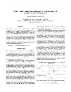
List of Figures and Tables Page Figure 1. 20 (A) Windowed waveforms (1 second before and 2.82 seconds after the catalog P pick) for two New Zealand earthquakes recorded at station MOW. The station sampling rate is 50 sample/sec and the signals are aligned by the P picks. (B) Windowed waveforms band-pass filtered between 1 and 6 Hz. (C, D) CC series for the (C) unfiltered (raw) and (D) filtered waveforms. (E,F) Bispectrum-correlation series for the (E) raw and (F) filtered waveforms. (G) Stacked raw waveforms. The upper trace is obtained by shifting the waveform of the first event with the CC determined lag relative to the second one, while the lower trace is computed after shifting the waveform of the first event with the lag calculated with the bispectrum method. The root-mean-square amplitudes for the two traces are 0.25 and 0.27 respectively. (H) Same as G for the stacked band-pass filtered waveforms. The root-mean-square amplitudes for the two traces are 0.32 and 0.34 respectively. Figure 2. 21 Examples of a) rejection of a high CC value due to inconsistent results between the CC and BS lags and b) acceptance of a low CC value due to consistent results between the CC and BS lags. Figure 3. Locations of 53 earthquakes near lake Wairarapa, NZ. (A) Before relocation; (B) relocated with catalog differential travel times; (C) relocated with CC differential travel times chosen with the threshold criterion; (D) relocated with CC differential travel times verified with the bispectrum method; (E) relocated with both catalog and threshold-chosen CC differential travel times; (F) relocated with both catalog and bispectrum-verified CC differential travel times.
22
Figure 4. Maps of (a) reference events and (b) test events and test stations from our California ground-truth dataset.
23
Figure 5. 23 Contour plots (map view and depth sections) of the maximum cross-correlation value per bin for the 7 stations for a test event (located at lat. 34.3', Ion. -118.58', and depth 1.8 km, cross) correlated against the set of reference events in the (a) lowfrequency band (step one) and (b) high-frequency band (step two). Note the good low-resolution location estimate on the left (circle) and the improved high-resolution location estimate (circle) on the right.
iv
24 Figure 6. Example application of KLD to a set of seismograms with a pair of "arrivals" only one of which is time-aligned across the records (top left), with noise added (top right). The data reconstructed from the 61 eigenvectors with eigenvalues above average in size (bottom left) retains both the time-aligned arrival and the arrival with moveout (middle left), leaving little signal energy in the residual image (middle right). In contrast, eigenimage decomposition cannot reconstruct both arrivals adequately. Figure 7. Example application of KLD to real data (upper left). Large and small eigenvalues were excluded in this case. The reconstructed data (upper right) from the 30 eigenvectors with eigenvalues from #5 to #34 (middle right) produces similar looking waveforms, leaving relatively little energy in the residual image (middle left). The eigenvectors for the larger eigenvalues (lower left) and their corresponding reconstructions (lower right) show the long-period noise character of the first 4 eigenvectors.
25
26 Figure 8. a,b) Seismic data windowed around the P arrival for the a) shallow (2 km) and deep (12 km) earthquakes from Northridge (S. California) cluster. The shallow event is used as the reference signal and the deeper event is used as the primary signal; noise has been added to the latter trace. c) Zero-lag cross-correlation between the primary and CANC-filtered traces for a range of signal alignments (see text). d) SNR for the CANC-filtered trace versus the error trace for a range of signal alignments. e) Common signal obtained from CANC adaptive filter. f) Error trace. Coherency filtering applied to data in a) and b) results in the signal traces displayed in g) and h), respectively. Figure 9. A horizontal slice through the true synthetic velocity model. The true velocity model in 3D is similar to a "vertical sandwich," with velocity constant with depth.
27
27 Figure 10. Event locations (filled circles) and stations (triangles) used for the synthetic data set. The inversion grid used in the standard and DD tomography solutions is shown as crosses. The inversion grid points are at X=-35, -15, 0, 2, 4, 6, 20, 35 km, at Y=-60, 40 -20, 0, 20, 40 km, and at Z=O, 3, 7, 11, 16 km. 27 Figure 11. Horizontal slices through the velocity models from (a) standard tomography and (b) DD tomography, and the difference between (c) the DD tomography solution and the true model and (d) the standard tomography solution and the true model. Black dots indicate the earthquake hypocenters within half the grid-size of the slice.
v
Figure 12. 28 Comparison of earthquake locations along the Hayward fault determined using (a) DD tomography, (b) DD location, (c) standard tomography, and (d) catalog data (no DD data). Each part shows a lat-lon plot (upper left) and zoomed-in plots (rotated to fault-parallel/fault-normal) of epicenters (upper right) and fault-normal (lower left) and fault-parallel (lower right) depth sections. Note how closely the hypocenters in panels a and b resemble each other, but with a systematic SW shift. The tight clustering is not evident in either the standard tomography solution (c) or the catalog locations using absolute picks only (d). Figure 13. 29 (a) The left-hand panels show fault-normal slices through the DD tomography model. The model has sharper features and a better correspondence between the main region of seismicity and the position of the sharp velocity contrast compared to the standard results in b. (b) The right-hand panels show fault-normal slices through the standard tomography model. The model has features that are less sharp and a poorer correspondence between the main region of seismicity and the position of the velocity contrast than the DD results Table 1. The absolute differences between the true locations and those from the DD location method based on 1D velocity model, standard tomography, and DD tomography.
vi
30
Summary Our research program consists of four components, each involving some aspect of multiple-event analysis: (1) high-precision waveform cross-correlation (WCC) for arrival time estimation, (2) robust event clustering, (3) waveform decomposition and source wavelet deconvolution reshaping, (4) double-difference (DD) multiple-event location and tomography. Our research focused initially on the development and testing of these seismic analysis methods using "ground-truth" datasets at different scales (local and regional), and was followed by the application of these methods to real-time and simulated real-time data streams. We completed the development and carried out initial testing of a multiple eigentaper algorithm for improved integer-sample WCC. This is an extension of the use of the eigentaper approach from the sub-sample to the integer-sample computations. Modifications have been made to the WCC code logic to provide the initial step for adaptation for multiple frequencyscale correlations. In addition, modifications have been completed to interface the WCC code with our new DD tomography code. This alters the code output to produce station correlations and lags on a by-event basis. We initiated an investigation of the use of multi-wavelet decomposition methods (in place of Fourier decomposition) for potential improvement of WCC. The initial findings were promising, but further assessment is required. Differential arrival times for pairs of seismic events observed at the same station are often calculated by WCC techniques. Researchers generally choose the differential times to use based on the associated cross-correlation (CC) values exceeding a specified threshold. When two similar time series are corrupted by correlated noise, the time delay estimate calculated with the WCC technique may not be reliable. Thus the selection of a threshold value is important. If it is set too high, then only a limited number of very accurate differential time data are available to constrain the relative positions of earthquakes. If the threshold value is set too low, then many unreliable differential time estimates are used and they will negatively affect the final relocation results. The bispectrum method can suppress the correlated Gaussian noise sources in two similar time series and be used to obtain the relative time delay between them. We compute time delay estimates between the waveform pairs with the bispectrum method and use them to verify the WCCdetermined one. This technique can provide quality control over the selected time delay estimates and potentially provide more differential travel time data for close events pairs, by verifying the reliability of differential times that might not meet the threshold criterion. A manuscript describing the technique and illustrating its application has been published (Du et al., 2004). We submitted the CC-bispectrum analysis code (BCSEIS) to our Product Integrator. We have tested two versions of a two-step event location technique with California and New Mexico ground truth (GT) data set. In step I of the first (UW) version, event locations are estimated via WCC of Hilbert-envelope waveforms. The Step 1 procedure accurately located the epicenters within 20 km (approximately I bin) of the NCSN catalog location for 16 of the 20 test events. However, depth estimates were poorly constrained. The Step 2 refinement based on WCC of the high-frequency P arrivals followed by DD relocation improved both epicenter and depth estimates. This two-step procedure offers advantages over conventional location techniques including a Step 1 event location not dependent on the accuracy of catalog picks and a Step 2 improvement in location accuracy using the high-accuracy DD technique. For the other I
(NMT) version, the approach is to find the most similar event from a reference database, and assign phases and location information of the most similar event in a reviewed database according to the spectrogram cross-correlation. No preliminary pick or location information is needed for the unknown event. Both approaches have proven effective in our trials. We developed a wavelet-based auto-picker for detecting and picking first-P arrivals that will be used in conjunction with our location processing procedures, both for identifying waveform segments for correlation and for adjusting stack picks. A manuscript describing the approach has been published (Zhang et al., 2003). We tested the potential of waveform reshaping methods using the California GT dataset. Two approaches were examined: an empirical deconvolution method and a deterministic depthbased method. The key to both methods is to determine an approach that "simplifies" the firstarrival wavelet but preserves the relative arrival time. We tested a variety of decomposition and filtering techniques with the multiple goals of noise reduction, waveform "homogenization" (reshaping to similar "wavelet"), and depth phase identification. Methods examined include eigenimage decomposition, Karhunen-Lo~ve decomposition (KLD), Correlated data Adaptive Noise Canceling (CANC), and coherency filtering. A key issue is the effect of arrival misalignment between a pair of traces on the success of a given technique. We tested a two-stage process whereby the similarity and strength of a CANC-filtered trace (relative to the original and error traces, respectively) is used to align the trace to the reference signal. We completed the development and testing of a 3D DD tomography code, starting from the DD location code hypoDD. We applied our new DD tomography algorithm, tomoDD, to a dataset from the Hayward fault, California, as an initial test to compare to previously published location results. We published a manuscript on the method and initial application (Zhang and Thurber, 2003). We also submitted the DD tomography code (tomoDD) to our Product Integrator. An additional version of the DD tomography code was subsequently developed, a spherical-earth version appropriate for regional-scale applications.
2
Introduction The standard processing approach for the determination of seismic event hypocentral locations involves a single-event procedure. Phase arrivals are timed and associated to define an event, and the associated phases are used (potentially along with arrival azimuths and slownesses) to compute a best-fitting location. It has been shown that order-of-magnitude reductions in event location errors and uncertainties are possible if multiple-event techniques are utilized. Recent studies of earthquakes in Hawaii (Rubin et al., 1998), California (Waldhauser et al., 1999), and at the Soultz geothermal area (Rowe et al., 2002b), and of explosions at the Balapan test site (Phillips et al., 2001; Thurber et al., 2001), and others, have demonstrated in a dramatic fashion the substantial improvement in the definition of seismogenic features or in the accuracy of relative locations of ground-truth events that is possible with multiple-event methods utilizing high-precision arrival-time estimation. The accuracy of event hypocenters is determined by several factors, including the network geometry, available phases, and arrival time accuracies (Pavlis, 1986). If more phases are available, the event hypocenters may be more stable. For example, S-wave phases will be very useful in constraining event depths and providing information that helps to decouple the hypocenters from the structure in the inversion (Gomberg et al., 1990). Due to the presence of noise, the arrival times picked either manually or automatically generally have errors. Recent studies have shown spectacular improvements in location precision for earthquakes and explosions when WCC and event clustering techniques are used to improve arrival time estimates or determine high-precision relative arrival times (VanDecar and Crosson, 1990). Such studies are based on the assumption that waves generated by two similar sources, propagating along similar paths, will generate similar waveforms, and WCC can then be used to determine precise relative arrival times. These studies have demonstrated substantial improvement in the definition of seismogenic features and in the accuracy of relative locations of ground-truth events that is possible using multiple-event methods with high-precision absolute or relative arrival-time data. Most seismic stations exhibit signal quality problems to some extent or another. When analyzing datasets that cover a wide geographic expanse and a wide magnitude range, any master station may at times have poorer signal quality than other sensors in a network, either because of clipping for a large, nearby event, or poor signal/noise for smaller, more distant ones. Reliance on a single station to perform all similarity choices is therefore not generally the best approach, and we are testing the success of a more adaptive technique where two or more stations may have their waveform similarity matrices compared for consistency, particularly among events that have been orphaned in the clustering step for one of the stations. Often the first arrival is very emergent and only later portions of the signal can be compared. In these cases, it is useful to have a sliding correlation window to search for similarity later in the event coda. We have performed interactive testing to demonstrate that sometimes highly similar events, whose first arrivals were uncorrelatable, can be well aligned using the secondary phases. One does not generally expect even among similar events that alignment of later phases will necessarily optimally align the first arrivals; however, among events whose similarity has been established at several correlation lengths for several stations, this provides a means of identifying arrivals at noisier stations and improving the ability to estimate hypocenters 3
for these events. We see this approach as a potential tool in generating autopicks at stations with poorer S/N; if a new event has been identified as belonging to a family of highly similar events, the pick for the poor station may be predicted based on its picks for better-recorded events in the same family, then the validity of the autopick may be verified (and its time adjusted) through comparing later, stronger portions of the waveforms. WCC analysis of P-wave data has shown the ability to identify event clusters based on the cross-correlation information. In a small study region, P wave data might suffice for identifying clusters and hence the source position. However, the smaller window lengths and high-frequency data used in WCC P-wave analysis limits the ability to construct unique location information in a larger study region. Shearer (1994) has demonstrated the use of low-frequency data (3 mHz to 0 0.1 Hz) for global event location and Withers et al. (1999) have successfully applied a similar method to local and regional data utilizing coarse and fine spatial grids. A hierarchical clustering analysis incorporating both the statistical advantages of cluster analysis with adaptive use of grid size and frequency content of the data set offers an alternate means to locate earthquakes. The order of magnitude reductions in location errors found with the use of WCC analysis for event clusters suggest a similar improvement can result from our hierarchical clustering analysis, with location accuracy limited mainly by the distribution of the ground truth (reference event) locations, binning interval, and the clustering statistics. Differential arrival times for pairs of seismic events observed at the same station are often calculated by WCC techniques. These differential times (or adjusted picks derived from them) can be used to improve dramatically the earthquake relocation results (Got et al., 1994; Dodge et al., 1995; Shearer, 1997; Rubin et al., 1999; Waldhauser and Ellsworth, 2000; Schaffet al., 2002). Researchers often choose the differential times to use based on the associated CC values exceeding a specified threshold. For example, Schaff et al. (2002) only selected those time delays with CC values larger than 0.7 and mean coherences above 0.7. The selection of an "optimum" threshold value is important but difficult. If it is set too high, then only a limited number of very accurate differential time data are available to constrain the relative positions of earthquakes. On the other hand, if the threshold value is set too low, then many unreliable differential time estimates are used and will negatively affect the final relocation results. Also the time delay estimate calculated with the CC technique may not be reliable when the noise sources in the two time series are correlated. The selection of an optimum threshold value is important but difficult. If it is set too high, then only a limited number of very accurate differential time data are available to constrain the relative positions of earthquakes. If the threshold value is set too low, then many unreliable differential time estimates are used which can negatively affect the relocation results. In our approach, we compute two more time delay estimates between the waveform pairs with the bispectrum (BS) method (the raw data and band-pass filtered data) and use them to verify the WCC-determined one using the band-pass filtered data. The BS method, which works in the third-order spectral domain, can suppress correlated Gaussian or low-skewness noise sources (Nikias and Raghuveer, 1987; Nikias and Pan, 1988). Du et al. (2004) adopt this method to calculate two additional time delay estimates with both the raw (unfiltered) and band-pass filtered waveforms, and use them to verify (select or reject) the one computed with the CC technique using the filtered waveforms. This technique can provide quality control over the 4
selected time delay estimates and potentially provide more differential travel time data for close events pairs, by verifying the reliability of differential times that might not meet the threshold criterion. The WCC approach and its variants work in the second-order spectral domain. When the underlying signal inside two similar time series can be regarded as a non-Gaussian process and the noise sources as zero-mean Gaussian processes, the similarities between the two time series can be better compared in the third-order or bispectrum domain (Nikias and Raghuveer, 1987; Nikias and Pan, 1988; Yung and Ikelle, 1997). This bispectrum method takes advantage of the fact that for Gaussian processes only all spectra of order higher than two are identically zero. Thus the effect of correlated Gaussian noise is completely suppressed when we compare the two time series in the bispectrum domain, while it may make WCC techniques fail to work well. Noise at a station for different events can be expected to be partially correlated due to a combination of constant predominant noise sources with time-varying amplitude (microseisms, wind or cultural noise) and site response effects. Cycle skips are another potential WCC pitfall that bispectrum analysis may help detect. In some situations, otherwise similar waveforms may be "contaminated" by some interfering signal (e.g., a depth phase) that may degrade their cross-correlation. In such circumstances, it would be desirable to be able to extract the underlying similar waveforms, filtering out the "noise" of the contaminating signal. A recent paper by Ulrych et al. (1999) reviews several decomposition and transformation techniques that are useful for signal-noise separation in an exploration seismic context. The two most relevant to our work are eigenimage decomposition and Karhunen-Lorve decomposition (KLD). KLD is distinguished from the more common eigenimage decomposition (essentially principal components) in that the latter extracts eigenvector-eigenvalue information from multi-channel data based on a covariance matrix computed at a single lag (zero), whereas the former carries out a decomposition for single-channel data based on a covariance matrix for multiple lags (Ulrych et al., 1999). In practice, to apply KLD to multi-channel data, an average covariance matrix can be computed. We can make an important distinction between the two fundamentally different ways WCC data has been used: (1) by directly using relative arrival times to determine relative event locations (e.g., Got et al., 1994; Waldhauser and Ellsworth, 2000), and (2) by adjusting absolute arrival time picks to minimize discrepancies among relative arrival times (Dodge et al., 1995; Rowe et al., 2002a). The advantage of the former approach is that it incorporates all the available information contained within the multitude of relative arrival time differences with a direct measure of quality (the correlation value) associated explicitly with each datum. A disadvantage is that some simplifying assumption needs to be made to derive the locations from the arrival time differences. For example, in the method of Got et al. (1994), the events in a cluster have precisely the same take-off angle and azimuth to each station. As a result, the derived locations are ultimately relative, not absolute, so that some assumption must be made to end up with useful event coordinates (e.g., final locations are computed relative to a catalog-based cluster centroid). Waldhauser and Ellsworth (2000) proposed a different location algorithm, in which the spatial partial derivatives for the set of events are evaluated at different reference points. Thus the absolute event locations are obtained, rather than the relative locations. It is assumed, however, that the path anomalies from velocity heterogeneity are location independent. This 5
assumption is valid for closely spaced events, but is not true for far apart events. As a result, the event locations are biased due to velocity heterogeneity (Wolfe, 2003). In contrast, the latter approach uses the relative arrival times to determine a much smaller number of adjusted arrival time picks, but these picks are absolute arrival times and so can be used to determine absolute locations (in an existing velocity model). We have developed a new algorithm that combines the advantages and avoid the disadvantages of the above approaches. It is based on the code hypoDD of Waldhauser and Ellsworth (2000), and makes use of both absolute and relative arrival time data. The method determines a three-dimensional (3D) velocity model jointly with the absolute and relative event locations. This approach has the advantage of including relative arrival times with their quality values along with absolute arrival times, thereby not discarding valuable information by only using adjusted picks, and at the same time dispensing with simplifying assumptions about ray path geometries or path anomalies and producing absolute locations, not just relative locations. Two versions have been developed, one Cartesian and the other spherical-earth. Methods, Assumptions, and Procedures High-precision waveform cross-correlation WCC can be a powerful tool for improving earthquake phase identification and subsequent hypocenter locations. Our software is being built upon an initial package that was designed to retroactively process large catalogues having existing phase picks (P and S). This package compares similar waveforms and identifies families of events meeting specified crosscorrelation thresholds, based on a master station or suite of stations. Within families of similar earthquakes, waveforms are compared on a station-by-station basis and their picks are adjusted by applying an L 1-norm based conjugate gradient technique to the matrix of first differences. Consistent, mean-adjusted picks are re-entered into trace headers for other uses such as waveform stacking, hypocenter location or seismic tomography. The process of time delay calculation and bispectrum verification can be briefly described as follows. For the k'th mutual station that provides waveforms for two earthquakes i and j, we rely on the catalog phase (P or S) picks to form the data windows used for time delay calculations. Then using the band-pass filtered waveforms, we calculate both the CC value CCijk and the relative time delay in lag number Aijk(cc) for the event pair. If the value of CCijk is larger than a threshold CCsub, we also perform sub-sample time delay calculation to get Aijk(sub) by a weighted linear fitting of the cross spectrum phase (Poupinet et al., 1984). After we make the CC calculations for all the mutual stations between events i and j, we can obtain the maximum CC value CCijmax for the event pair. If CCijmax is larger than a second threshold CCbs, we will perform
bispectrum time delay estimation for each mutual station of the event pair. We obtain two estimates of time delay in lag number, i.e. Aijk(bs1) using the band-pass filtered waveforms and Aijk(bs2) with the raw waveforms. Thus depending on the extent of waveform similarity for an event pair, which is measured by the size of CCij"ma, four possible time delay estimations are carried out at a mutual station for either P or S waves.
6
Besides the aforementioned threshold value that researchers often use to select time delay estimates, which we term CC"iml, three other parameters CClim2 , CClim3 and Alim control the bispectrum verification process. Generally CClim2 ; CCliml a CClim3 . After we make the CC calculations across all the mutual stations of an event pair, we compare the maximum CC value CCijmax with CClim2 . If CC1 jmaX is larger than CClim2 , we will verify the CC time delay estimates for those stations with CCjk larger than CCHim 3 . A CC time delay estimate Aijk(cc) is trusted (or passes the verification) if its differences from both A1jkbl) and Aij kbs2), the ones determined with the bispectrum method, do not exceed the tolerance limit Aim. In other words, for an event pair with high CCijm"a value we will select the CC time delay estimates as long as they pass the bispectrum verification, even though the CC values associated with some of them are smaller than CC"Im" and would not be used under the threshold criterion often adopted by other researchers. If CC"m`1 5 CCij max < CClira2, we will make the verifications only for those stations with CCjk larger than CCliml. If CCqImax falls below CCliml, the CC time delays for the event pair are simply discarded. As an example, we apply this technique to obtain bispectrum-verified WCC differential times for a set of New Zealand earthquakes, and relocate 521 of the events using the DD algorithm hypoDD (Waldhauser and Ellsworth, 2000). We find that the bispectrum-verified time delays provide more clustered earthquake relocation results with lower arrival time residuals compared to the threshold criterion. We do not claim that the BS method always obtains a better time delay estimate than the CC technique. Rather, we use the BS time delay estimates to check the reliability of the ones computed with the CC technique. By applying two different methods that work in different spectral domains (second- and third-order), we can improve the reliability of the selected time delays. Generally for an earthquake, fewer S arrivals are available in the phase catalog than P arrivals because they are more difficult to select. We can obtain additional bispectrum-verified S differential times for those waveforms lacking catalog S picks, using the predicted S arrivals either from a velocity model (Shearer, 1997) or from the S-P time of a nearby event. Our work demonstrates that relocation results can be further improved with these additional time constraints. Event clustering We tested the clustering strategies applied with the agglomerative, dendrogram-based clustering algorithm of Rowe et al. (2002a), applying variable correlation window lengths and targeting different parts of the waveform in tiered clustering and sub-clustering processes. We have found substantial success in correlating on the later parts of a waveform rather than on the first arrival in some instances, as signal-to-noise of the first-P arrival can be low for emergent or nodal arrivals. Our NMT and Sandia collaborators finalized the New Mexico GT dataset for our detailed clustering and real-time tests. The New Mexico dataset consists of two parts, one spanning July 1997-February 1998 (Dataset A) that has undergone a complete repicking, relocation, WCC, and
7
clustering analysis, and the other spanning January 2001-December 2002 (Dataset B) that was prepared for real-time testing. We have implemented and tested a two-step clustering/location technique that offers several advantages over conventional techniques due to its use of WCC and DD location methods. Step 1 event clustering is based solely on high-quality GT event waveforms without use of catalog picks. Step 2 location estimates offer the same improvement in location accuracy as documented by the use of high-resolution DD techniques over standard techniques (Waldhauser and Ellsworth, 2000). We evaluated the technique using 640 events from Northern California (magnitude range 4.3-5.3) using a 60 x 6' study region and 7 master stations from the UC Berkeley seismic network (Figure 3). In step 1, event cluster locations are estimated via CC of Hilbert-envelope waveforms. A test event is cross-correlated against a suite of reference events binned by latitude, longitude, and depth. The step 1 location derived from the CC global maximum is then used as a starting location in the step 2 refinement using the DD relocation method (hypoDD). We initially carried out testing of our hierarchical (multiple-frequency-band) clustering/WCC analysis on a California GT dataset that we constructed specifically for such testing purposes. The dataset consists of waveforms for 697 events with magnitude 4 and above from central and northern California. We affirmed the quality of the GT location information by carrying out a DD location analysis. Relocation with hypoDD using NCSN data from 25 Berkeley network stations provided GT hypocenter information for the test events. We explored 4 different parameter settings controlling the extent of clustering and residual outlier rejection. We found that the DD locations reproduced those in the catalog within 2 to 3 km (in epicenter and depth) on average. Then the dataset was divided into two parts, consisting of 162 "master" events (the largest in each location bin) and the remainder as "test" events. An adaptive, automatic phase-picking and epicenter-locating program is now fully developed and is being applied to update the New Mexico microseismicity catalogue. The programoperates in the MATLAB environment (on the UNIX platform) under MatSeis (developed by Sandia National Laboratories). The package is named PLRR (Pick-Locate-RepickRelocate). The approach of PLRR is to find the most similar event from a reference database, and assign phases and location information of the most similar event in a reviewed database according to the spectrogram cross-correlation. No preliminary pick or location information is needed for the unknown event. Some characteristics of the PLRR package, which will be submitted to our Product Integrator, are: 1. Data format. The seismic data format recognized by PLRR is the CSS-3.0 flatfile format. 2. Reference database. The quality of phase-picking and epicenter-location results will ultimately depend on the coverage and quality of the reference database. 3. Spectrogram waveform cross-correlation. We find the phase character for this data set is most diagnostic and discriminates events best within a limited bandwidth between 6 and 10 Hz.
8
4. Waveform-pair match and event-pair match. We have explored two options in PLRR to find phases and locations for unknown events. The first one, waveform-pair matching, finds the most similar waveforms in the reference database relative to all waveforms, station by station, and assigns the corresponding respective phase information to the new waveforms. This technique was found to produce too many false associations. The second one, event-pair matching, is more robust. This option stacks the CC coefficient curves of waveform-pairs between the unknown event and waveforms grouped from each event in the reference database, and finds the reference event which has the highest stacked CC coefficient value (by taking the mean/median of stacking CC coefficient curves) as the most similar event to the unknown event. 5. Database Operation. Several simple functions to enhance and simplify the operation of CSS3.0 database are added into PLRR, such as the "Update monthly table," which add new event to a CSS-3.0 database. Waveform/wavelet analyses We developed a wavelet-based auto-picker for detecting and picking first-P arrivals that will be used in conjunction with our location processing procedures, both for identifying waveform segments for correlation and for adjusting stack picks. A manuscript describing the approach is in the final stages of preparation. Once we completed the construction of the California GT dataset, we began to test potential waveform reshaping methods using this GT dataset. Two approaches are being examined: an empirical deconvolution method and a deterministic depth-based method. The key to both methods is to determine an approach that "simplifies" the first-arrival wavelet but preserves the relative arrival time. We tested a variety of decomposition and filtering techniques with the multiple goals of noise reduction, waveform "homogenization" (reshaping to similar "wavelet"), and depth phase identification. Methods examined include eigenimage decomposition, Karhunen-Lodve decomposition (KLD), Correlated data Adaptive Noise Canceling (CANC), and coherency filtering. A key issue is the effect of arrival misalignment between a pair of traces on the success of a given technique. We tested a two-stage process whereby the similarity and strength of a CANC-filtered trace (relative to the original and error traces, respectively) is used to align the trace to the reference signal. Double-difference tomography We have developed a new DD tomography method (Zhang and Thurber, 2003), which takes the DD location method (Waldhauser and Ellsworth, 2000) a step further to solve for 3D velocity structure simultaneously with hypocenter locations using both catalog picks and differential arrival times (WCC and catalog). At the local scale (10s to 100s of kilometers), the earth can be represented with a flat model. We use the pseudo-bending ray-tracing algorithm (Um and Thurber, 1987) to find the rays and calculate the travel times between events and stations. The model is represented as a regular set of 3D nodes and the velocity values are interpolated by using the tri-linear interpolation method. The hypocenter partial derivatives are calculated from 9
the direction of the ray and the local velocity at the source. The ray path is divided into a set of segments and the model partial derivatives (calculated in terms of fractional slowness perturbation, so that the derivatives are related to path length) are evaluated by apportioning the derivative to its 8 surrounding nodes according to their interpolation weights on the segment midpoint (Thurber, 1983). The body wave arrival time T from an earthquake i to a seismic station k is expressed using ray theory as a path integral Tk ==It• +f.ku ds (1) where Ti is the origin time of event i, u is the slowness field and ds is an element of path length. The source coordinates (xl, x2, x3), origin times, ray-paths, and the slowness field are unknown model parameters. The relationship between the arrival time and the event location is nonlinear, so a truncated Taylor series expansion is generally used to linearize Equation (1). The misfit between the observed and the predicted arrival times can be linearly related to the perturbations to the hypocenter and velocity structure parameters r a•T• i = -.--4iAx, +Ati + fkbu ds
(2)
1=1 ax I
If we subtract from Equation (2) an equivalent equation for event j, we have
aV 0T r-
0rk=
_
k•
2s !1 0X1I Axl +At
+ fku ds
j
J-Tk
1=1
xI
k
-A
-
6u ds
(3)
Assuming that these two events are near each other so that the paths from these two events to the common station are almost identical and the velocity structure is known, then Equation (3) can be simplified as k
k
=
-
aTj
a~k'
Ax +At Ix-;
-i
-
a,,xj k _Atd
(4)
Use of Equation (4) is known as the "double-difference" (DD) earthquake location algorithm (Waldhauser and Ellsworth, 2000). Wolfe (2003) has carried out an elegant comparison of this method to those of Jordan and Sverdrup (1981) and Got et al. (1994), pointing out the general similarities and subtle differences, and discussing the advantages and limitations of each method. Her most important conclusion is "that when the path anomalies from velocity heterogeneity change strongly with earthquake position, the bias effects can be reduced in the relative locations between closely spaced earthquakes, but the effects cannot be reduced in the relative locations between earthquakes spaced far apart." Two assumptions in the Waldhauser and Ellsworth (2000) method are key: an a priorilayered velocity model is assumed, and they add a constraint equation forcing the mean shift of all earthquakes to be (approximately) zero.
10
We can generalize the 3D DD location method to jointly determine the 3D velocity structure and the (absolute) event locations. The equations for the DD tomography algorithm, tomoDD, are: _uJsAtJ
r+-rdi At k • axI
1=1
aT' -
i
k~f
xAxi +Ati +
J
I
d
k!
(5)
8u ds
Our tomography algorithm incorporates first-difference smoothing constraints, with a greater smoothing constraint weight applied to horizontal direction than the vertical (since vertical velocity changes are generally expected to be greater). At the regional scale (100's to 1000's of km), the earth should not be treated as flat, but as a sphere. Some velocity discontinuities such as Conrad, Moho, and subducting slab boundary should also be taken into account. Finite-difference ray tracing algorithms developed by both Podvin and Lecomte (1991) and Hole and Zelt (1995) are able to accurately calculate first-arrival times in the presence of extremely severe, arbitrarily shaped velocity discontinuities. These algorithms solve a finite difference approximation to the Eikonal equation in the regularly gridded velocity structure through a systematic application of Huygens' principle. This procedure can explicitly take into account different propagation modes including transmitted and diffracted body waves, and head waves in addition to direct waves. The principle of reciprocity is utilized by placing the source point at the seismic station location and interpolating the travel times computed at the grid nodes to match the exact earthquake location (Flanagan et al., 1999). To adapt the finite-difference algorithm to the regional scale, the curvature of the Earth must be taken into account. Earth flattening transformation is only valid for 1D velocity models and not for 3D velocity models. Following Flanagan et al. (2000), we solved this problem by parameterizing a spherical surface inside the Cartesian volume of grid nodes. The coordinate center was put at the surface of the Earth, positive X and Y-axes point to the direction of North and West, and positive Z-axis points downward, respectively. The grid nodes above the Earth surface (air nodes) are attributed to the true velocity values traveling in the air. As a result, all the rays travel inside the Earth. The regular uniform velocity (slowness) grid nodes used to calculate the travel time field using finite-difference algorithms are interpolated from the non-uniform inversion grid nodes through tri-linear interpolation. If an inversion grid node is 2 km above the Earth's surface, then it is treated as an air node and its value is fixed during the inversion. We treat each station as a source and calculate travel times to all velocity nodes in the volume. The travel time from a station to each earthquake is interpolated from its 8 neighboring nodes through trilinear interpolation. The ray path from the earthquake to the station is found iteratively with increments opposite to the travel time gradient. After these steps, DD tomography is adapted to the regional scale with ray paths and related partial derivatives calculated by the finite-difference method.
11
Results and Discussion High-precision waveform cross-correlation The WCC program has some features that help it to perform in an auto-adaptive manner. These include: adaptive, full-spectrum cross-coherency-based prefiltering; a multi-component signal covariance estimator that provides automatic, adaptive polarization filtering to optimize signal linearity; and the use of multiple eigentapers in the subsample cross-spectral correlation step to reduce signal leakage and variance when estimating the signal cross-spectra. We have adapted the cross-correlation program with the addition of eigentapers in the coarse (integersample) cross-correlation step, and we are in the process of comparing this approach to coarse lag estimation with the previous method of applying multiple narrow-band filtering. Both approaches provide a means of estimating linearly independent realizations of the time series and therefore permitting quantitative error estimates for the integer correlation step; in future work we will combine the two strategies via application of multiple eigenwavelet methods. The correlator has also been adapted so that its output may optionally be generated in a format that is compatible with the hypoDD program, so that joint location may be performed using the cross-correlation comparisons without actually solving for consistent pick lags and correcting the picks themselves. Further, the correlator now has an option of generating only one set of first-differences, for applications in which it is only desired to compare a set of "reference events" to the trace of a single ("test") event. This option is being tested in our hierarchical approach described in the next section. Figure 1 demonstrates the application of the CC and bispectrum methods to the waveforms of two closely spaced M2.5 New Zealand earthquakes. The waveforms for these events recorded at nearby stations are highly similar, but the signal to noise ratios (SNRs) for the records at station MOW (epicentral distance of 93 km) are noticeably lower (Figs. 1A and IB). The two bispectrum-correlation series (Figs. IE and IF) peak at lag 6 and 7 respectively, whereas the two CC series (Figs. IC and ID) reach maxima at lags very different from each other and also from the two bispectrum-correlation series. Careful examination reveals that the two CC series reach local maxima at lag 7. They fail to become global maxima there, however, apparently due to the contamination of correlated noise. Figures 1G and IH plot the stacked signals for both raw and band-pass filtered waveforms. In both cases the lower trace (the stacked signal obtained by shifting the waveform of the first event with bispectrum-determined lags) has a larger root-meansquare (RMS) amplitude than the upper trace, which is obtained after shifting the waveform of the first event with the CC-determined lags. The above example corroborates the findings of Nikias and Pan (1988) and Yung and Ikelle (1987) that the bispectrum method works better than CC techniques in getting relative time delay between two similar signals contaminated by correlated noise. Figure 2 shows examples of the application of the BS verification method to waveforms recorded at New Zealand stations for two pairs of relatively close events. In Figure 2a, the CC value (0.74) is above the nominal threshold (0.70), but the lag does not agree with that obtained from BS (bottom panel), so this CC value is rejected. From the seismograms, we can see that this is apparently a case of cycle skipping - the filtered waveforms coincidentally correlate slightly 12
better at a lag of-10. In Figure 2b, both methods provide the same time delay, but the associated CC coefficient is only 0.50. Under the threshold criterion, such a time delay estimate associated with a low CC coefficient is simply discarded. Using the BS checking method, however, we can identify the reliable time delays from these "seemingly not very similar" waveforms, such as for this pair, and as a result provide more control over the relative locations of the events. Du et al. (2004) apply this technique to 822 New Zealand earthquakes in the Wellington area and find that the CC time delays verified with the BS method provide improved earthquake relocation results (noticeably more clustered) compared to those selected with the standard threshold criterion. An example of the improvement of the BS-verified locations compared to original catalog locations, DD locations using differential catalog picks, and DD locations using standard threshold CC lags is shown in Figure 3 for a sub-region near Lake Wairarapa, NZ. Event clustering Waveform clustering, used to segregate signals in to families of similar events, has been tested with a variety of approaches. One successful approach has been to identify clusters based on very high standards of cross-correlation (0.8 or 0.85), resulting in many small multiplets of highly similar events. These are then cross-correlated and consistent pick adjustments are determined via a conjugate gradient solver. Waveforms are aligned on their new picks and stacked to provide a composite waveform representation for the cluster. These stacks are then crosscorrelated among the multiplets and inconsistencies in the mean adjusted picks can be corrected by finding consistent adjustments among the stacks. The resulting stack pick lags are propagated to the parent traces. This has been shown to reduce the inter-cluster inconsistencies that result in cluster centroid biases when earthquakes are located using the new picks (these biases existed in the initial catalogue as well). Another related approach that has shown good success is application of the clustering program to the waveform stacks. Those traces whose stacks cluster together based on a high similarity coefficient are joined into larger, second order families. Their member traces are cross-correlated and adjusted for consistency within this larger group. The second-order clusters, following pick adjustment, are stacked yet again and their stacks are compared for similarity. This process may be performed in a hierarchical manner until stacks fail to cluster. Final adjustment of mean centroid picks on the ultimate stacks has been tested using an autopicker; this works well when many traces contribute to the stack but we are still testing different methods of estimating pick uncertainty from the autopicker functions. Phase-weighted stacking, jackknifing methods or multiple-frequency-band approaches may provide the best uncertainty estimates. We constructed two regional ground-truth datasets, one for New Mexico and one for California. The former dataset is from the New Mexico Tech short-period network and is dominated by small explosions, whereas the latter is from the UC-Berkeley broadband network and contains relatively large earthquakes. The New Mexico dataset consists of two parts, one spanning July 1997-February 1998 that has undergone a complete repicking, relocation, WCC, and clustering analysis, and the other spanning January 2001-present that is being prepared for real-time testing. The California dataset was extracted from the Northern California Earthquake Data Center (NCEDC). We first affirmed the quality of the NCEDC catalog location information 13
by carrying out a DD location analysis using catalog time-difference data for 130 events and 23 stations. We found that the DD locations reproduced those in the catalog within 2 to 3 km (in epicenter and depth) on average. We then used a combination of automatic and manual picking to augment and improve the available P arrival picks, and to provide analyst pick weights. We present the results of hierarchical WCC/clustering analysis on the California GT dataset, based on WCC analysis of P through surface waves in a first step and the P phase in a second step. We binned the events in 0.10 latitude and longitude bins and in 2.5 km depth bins. The largest magnitude events per bin comprise our 162 reference events, and the next largest 24 events are used for the test dataset. The reference events are displayed in Figure 4a, and the test events and stations used for the preliminary hierarchical analysis are shown in Figure 4b. The WCC analysis for the two steps was accomplished in a similar manner. Waveform data from each test event were cross-correlated against the reference event waveforms to determine the maximum value, in the whole region using low-frequency data in step one, and in a 20 region about the stepone location estimate using high-frequency data in step two. The maximum cross-correlation value per bin from the 7 stations was contoured as an indicator of test event location. Figures 5a and b display the results for a test event located near Los Angeles. For this example, the WCC analysis is performed on the vertical component data for both steps. The estimated location for this event falls with 25 km of the catalog location using the low-frequency data, and improves to 7.5 km using high-frequency data. We then tested the two-step event location technique with a California GT data set. We augmented the existing P and S picks from the network catalog using skew and kurtosis analysis followed by a manual evaluation. Many catalog P picks required manual adjustment. We then prepared WCC data based on 3- and 5-second P windows (Rowe et al., 2002a). In step 1, event locations are estimated via WCC of Hilbert-envelope waveforms. The entire seismogram was filtered and an eigenvector decomposition of the covariance matrix was applied to the 3component data (Rowe et al., 2002a) prior to the calculation of Hilbert-envelopes for the principal direction. Test event data for each of the master stations were cross-correlated against 161 GT events with the position of the CC global maximum determining the step 1 location (Figure 3). The Step I procedure accurately located the epicenters within 20 km (approximately 1 bin) of the NCEDC catalog location for 16 of the 20 test events. However, depth estimates were poorly constrained. The Step 2 refinement based on WCC of the high-frequency P arrivals followed by DD relocation improved both epicenter and depth estimates. For each test event, subsets of the catalog and WCC data are prepared for use in hypoDD with the step 1 location providing the initial test-event location. This two-step procedure offers advantages over conventional location techniques including a Step 1 event location not dependent on the accuracy of catalog picks and a Step 2 improvement in location accuracy using the high-accuracy DD technique. We submitted the automated two-step location code (PLRRUW) to our Product Integrator. Waveform/wavelet analyses We tested a variety of decomposition and filtering techniques with the multiple goals of noise reduction, waveform "homogenization" (reshaping to similar "wavelet"), and depth phase 14
identification. Methods examined include eigenimage decomposition, Karhunen-Lodve decomposition (KLD), Correlated data Adaptive Noise Canceling (CANC), and coherency filtering. A key issue is the effect of arrival misalignment between a pair of traces on the success of a given technique. Some methods rely on signals being time-aligned before processing, which of course cannot be assumed for seismic data in a monitoring context. We also developed a waveletbased auto-picker for detecting and picking first-P arrivals that can be used in conjunction with our location processing procedures, both for identifying waveform segments for correlation and for adjusting stack picks (Zhang et al., 2003). We have been testing the utility of the KLD method for extracting similar signals from noisy data. A synthetic example is shown in Figure 6. In this particular case, we construct initially noise-free seismograms (upper left panel) that consist of a first-arriving signal that is time-aligned and an identical second-arriving signal with substantial moveout. Gaussian noise with RMS amplitude 20% of the signal amplitude is added (upper right panel) and eigenimage decomposition (not shown) and KLD are carried. The eigenimage decomposition, using eigenvalues of average value and greater, preserves the time-aligned signal but degrades the secondary arrival, leaving most of the latter's energy in the residual "noise." KLD (middle left panel), again using eigenvalues of average value and greater (bottom left panel), preserves both the time-aligned signal and the secondary arrival (middle right panel). For a second example, we apply KLD to real data from a group of earthquakes of magnitude 3.6 to 3.8 in Long Valley, CA, from January 1998. In the catalog, the events are within about 1 km of each other in epicenter but have estimated depths ranging from 0.5 to 5.0 km. Relocation using hypoDD and catalog arrival times plus catalog-generated arrival time differences yields epicenters within less than 1 km and depths within 250 m of each other. The analyzed waveforms were recorded at station ORV with an epicentral distance of 314 km. The results of the KLD analysis are shown in Figure 7. The raw data traces are relatively noisy. In this case, we recognize that the eigenvectors for the four largest eigenvalues represent long-period noise (bottom left panel), and we exclude them along with the smaller eigenvalues. The resulting KLD-processed traces (upper right panel) are quite similar and the data residue (middle left panel) contains no obvious remnant signal of interest. In contrast, the eigenimage decomposition does little if anything to improve the signal similarity, only removing some of the higher frequency noise. An alternative approach to noise reduction via extracting common waveform signals is adaptive filtering. We have experimented with a CANC algorithm of Hattingh (1988). Input into the CANC procedure consists of a "reference signal" SI and a "primary signal" S2, correlated to each other in some unknown way. Each signal is presumed to contain noise that is uncorrelated with the noise from the other trace. The reference signal is used as a "learning signal" to derive filter coefficients. The filter adjusts its impulse response to minimize the mean-squared error between filter output and the primary signal (in terms of power). The algorithm rapidly solves for the filter coefficients without requiring matrix inversion or a CC operation. The CANC procedure is an iterative solution, computing updated filter coefficients at each iteration. We apply the CANC procedure to seismic data from two events in a cluster with similar catalog epicenters but different depths, recorded at UC-Berkeley network station SAO. The two events are from the 1994 Northridge aftershock sequence and are located within 7 km of each 15
other in epicenter based on catalog information. Trace I (Figure 8a), the reference signal, is from a shallow earthquake (2 km depth), whereas trace 2 (Figure 8b), the primary signal, is from an earthquake occurring at greater depth (12 km). We apply adaptive filtering to shape the windowed signal from the deeper earthquake to extract the signal common to the shallow event in an attempt to improve subsequent WCC results. We use a 7 s window containing approximately 4.5 s of data following the P pick. The windowed signal from the deeper event (Figure 8b) was aligned relative to the shallow event signal (Figure 8a) initially by the P picks and then fine-tuned by applying a lag search. The zero-lag CC between the primary and filtered traces (Figure 8c) and the signal-to-noise ratio of the filtered trace relative to the error trace (Figure 8d) have coincident maxima. After 5 iterations of the CANC algorithm, the signal from the deeper event is successfully decomposed into an estimate of the common signal (Figure 8e) and the dissimilar error signal (Figure 8f). We can compare the estimate of common signal to individual trace output by the application of coherency filtering. Shown are the coherency-filtered traces for the shallow and deep event (Figures 8g and h). The frequency content of the two clustered events is very similar as might be expected. Consequently, coherency filtering yields output traces similar to the original trace data. The adaptive filter shaping of the deep event's waveform visually yields a signal (Figure 8e) closer in appearance to the shallow event (Figure 8a). Application of adaptive filtering increases the maximum CC value for the shallow event with the CANC-filtered trace from 0.51 to 0.83. CC of the coherency-filtered data yields a maximum value of 0.70. These CC maxima occur at the same lag. Thus the CANC approach can successfully extract a more similar waveform from the primary signal than coherency filtering while preserving timing. Double-difference tomography We have tested the local-scale version of DD tomography (tomoDD) with a synthetic dataset that was constructed on the basis of an idealized model of the velocity structure of the San Andreas Fault in central California (Kissling et al., 1994) shown in Figure 9. The events and stations used to construct the synthetic dataset are from the actual seismicity and USGS stations in the Loma Prieta region (Figure 7). We added Gaussian random noise with zero mean and a standard deviation of 0.04 s to all the true arrival times. In addition, we also added a constant noise term to the arrivals at each station from a uniform distribution between -0.3 s and 0.3 s. This simulates the case that the systematic errors (model errors and pick bias) associated with the arrival times are larger than the random ones. We construct the pseudo "cross-correlation" data directly from the absolute arrival times by differencing the synthetic arrival times at common stations for events pairs within 20 km. As a result, the "cross-correlation" data are more accurate than the absolute data. We first use the DD location algorithm hypoDD to relocate the events (Waldhauser, 2001). The 1D velocity model used is the Dietz and Ellsworth (1990) model, based on seismic refraction and earthquake data. We use both the residual weighting and distance weighting schemes in the inversion to control the large residuals, as did Waldhauser and Ellsworth (2000). The absolute differences between this set of event relocations and the true locations and their standard deviations are shown in Table 1. The results indicate that the event relocations from the 16
DD location algorithm based on a ID velocity model have a substantial bias (>1 km in each coordinate direction) from the true locations. This bias is caused by a difference between the velocity model (horizontal layers) used to calculate the DD locations and the true velocity model (vertical "sandwich") used to generate the data. The heterogeneity of the true velocity model makes path anomalies different for different events. However, the DD location method assumes that the path anomalies are location-independent, and this assumption introduces bias into event locations (Wolfe, 2003). Next, we show the results of applying the standard tomography method to the relatively noisy absolute arrival times. The inversion starts from the same ID velocity model as the DD location method. The X-Y nodes used to represent the velocity model are shown in Figure 10; in depth, nodes are positioned at 0, 3, 7, 11, and 16 km. The computational algorithm is identical to that for DD tomography, but the differential times are excluded. Both damping and smoothing (with weight 5.0 in both the horizontal and vertical directions) are applied to the inversion to make the solution more stable. Figure 8a shows horizontal slices through the velocity structure obtained from the standard tomography. The absolute difference between this velocity model and the true velocity model has a median value of 0.164 km/s, a mean value of 0.245 km/s and a standard deviation of 0.249 km/s. The main features of the true velocity model are evident in the depth slices. The event locations have smaller errors than those from the DD location method (Table 1). DD tomography uses both the noisy absolute arrival times and more accurate differential times. We also apply damping and the smoothing constraints to stabilize the solution, with the residual weighting used to penalize the large residuals during the inversion. DD tomography starts with the same 1D velocity model and uses the same inversion grid as the standard tomography. Figure 11 a and b shows the horizontal slices of the velocity structure from conventional and DD tomography. The absolute difference between the DD tomography velocity structure and the true velocity structure has a median value of 0.136 km/s, a mean value of 0.178 km/s, and a standard deviation of 0.164 km/s, compared to a median value of 0.164 km/s, a mean value of 0.245 km/s, and a standard deviation of 0.249 km/s for conventional tomography. DD tomography characterizes well the low velocity zone of the true velocity model, especially at the depths of 3 km and 7 km. Subtracting the DD tomography solution and the standard tomography solution from the true model (Figure 11 c and d), we find that the velocity model from DD tomography has a more correct value in the low-velocity trough except at the depth of 0 km, where the ray paths from event pairs almost completely overlap and the accuracy of velocity structure is mainly controlled by absolute catalog data. This indicates that DD tomography recovers better the low-velocity zone, and overall the velocity model is more accurate than the standard tomography. Compared with the standard tomography method, DD tomography also produces more accurate event locations (Table 1). Conclusions and Recommendations Advances in techniques for waveform alignment, event clustering, waveform decomposition, and location and tomography have been achieved with the support of this contract. We echo the conclusion voiced by Prof. Paul Richards that a quantum change is needed 17
in the manner in which earthquake locations are determined in the seismic monitoring environment (both nuclear and otherwise). Effective tools for event clustering, waveform alignment, and joint location/tomography are available, and a concerted effort will be required to implement these tools in "real-world" monitoring situations. Accomplishing this will probably require closer and more direct interaction between the tool developers and the users, in particular to allow for direct feedback from the users to the developers. Differential arrival times for pairs of seismic events observed at the same station are often calculated by WCC techniques. Researchers often choose the differential times to use based on the associated cross-correlation (CC) values exceeding a specified threshold. When two similar time series are corrupted by correlated noise, the time delay estimate calculated with the WCC technique may not be reliable. Thus the selection of a threshold value is important. If it is set too high, then only a limited number of very accurate differential time data are available to constrain the relative positions of earthquakes. If the threshold value is set too low, then many unreliable differential time estimates are used and they will negatively affect the final relocation results. The bispectrum method can suppress the correlated Gaussian noise sources in two similar time series and be used to obtain the relative time delay between them. We compute time delay estimates between the waveform pairs with the bispectrum method and use them to verify the WCCdetermined one. This technique can provide quality control over the selected time delay estimates and potentially provide more differential travel time data for close events pairs, by verifying the reliability of differential times that might not meet the threshold criterion. WCC is vulnerable to problems associated with correlated noise that can be overcome using bispectrum analysis. It is our recommendation that a verification approach comparable to that described here be adopted for earthquake location applications for which very high accuracy is essential. A hierarchical location approach, for "new" events relative to a set of reference events, that starts with CC of long records at low frequencies to identify the approximate source region based solely on waveform or spectrogram similarity and then switches to single-event or DD location using CC of short records at high frequencies works effectively for our regional datasets. We have tested two versions of a two-step event location technique with California and New Mexico GT data set. In step 1 of the first (UW) version, event locations are estimated via WCC of Hilbert-envelope waveforms. The Step 1 procedure accurately located the epicenters within 20 km (approximately 1 bin) of the NCSN catalog location for 16 of the 20 test events. However, depth estimates were poorly constrained. The Step 2 refinement based on WCC of the highfrequency P arrivals followed by DD relocation improved both epicenter and depth estimates. This two-step procedure offers advantages over conventional location techniques including a Step 1 event location not dependent on the accuracy of catalog picks and a Step 2 improvement in location accuracy using the high-accuracy DD technique. For the other (NMT) version, the approach is to find the most similar event from a reference database, and assign phases and location information of the most similar event in a reviewed database according to the spectrogram cross-correlation. No preliminary pick or location information is needed for the unknown event. Both approaches have proven effective in our trials. This approach should next be tested in a real-time monitoring environment.
18
We tested a variety of decomposition and filtering techniques with the multiple goals of noise reduction, waveform "homogenization" (reshaping to similar "wavelet"), and depth phase identification. The KLD and CANC methods show the most promise for allowing the isolation of similar underlying waveforms that are not time-aligned. We have developed the new method of DD tomography. The inversion code tomoDD takes the double-difference location method (hypoDD) a step further to solve for 3D velocity structure simultaneously with hypocenter locations using both catalog picks and differential arrival times (WCC and catalog). Compared to conventional tomography, the result is a sharpening of the seismicity distribution equal in quality to hypoDD plus a sharpening of the velocity image due to removal of the majority of the location scatter. We have developed localand regional-scale versions of tomoDD, and have applied each to synthetic and real datasets. Synthetic tests show the method yields locations with greater accuracy than either DD location or standard tomography, and a velocity model that is closer to the true model than standard tomography. The DD tomography approach works with either waveform-based or catalog-based differential time data, and thus is applicable to any dataset to which standard tomography can be applied. ACKNOWLEDGEMENTS We thank Megan Flanagan for providing codes for the spherical earth finite-difference method and Charlotte Rowe for many valuable discussions. We also thank Haijiang Zhang, Wayne Du, Bill Lutter, Jean Battaglia, Rick Aster, and Wenzheng Yang for their contributions to this report.
19
Figure 1. (A) Windowed waveforms (I second before and 2.82 seconds after the catalog P pick) for two New Zealand earthquakes recorded at station MOW. The station sampling rate is 50 sample/sec and the signals are aligned by the P picks. (B) Windowed waveforms band-pass filtered between 1 and 6 Hz. (C, D) CC series for the (C) unfiltered (raw) and (D) filtered waveforms. (E,F) Bispectrum-correlation series for the (E) raw and (F) filtered waveforms. (G) Stacked raw waveforms. The upper trace is obtained by shifting the waveform of the first event with the CC determined lag relative to the second one, while the lower trace is computed after shifting the waveform of the first event with the lag calculated with the bispectrum method. The root-mean-square amplitudes for the two traces are 0.25 and 0.27 respectively. (H) Same as G for the stacked band-pass filtered waveforms. The root-mean-square amplitudes for the two traces are 0.32 and 0.34 respectively.
20
Windowed Waveforms (OTW; 50 sp/sec; filtered)
Windowed Waveforms (KIW; 50 sp/sec; filtered)
100
oso
0
ISO
Cross-Correlation Series (lag : -10; max = 0.74) 10t
1.0,
100
150
Cross-Correlation Series (lag =0; max
=
0.50)
0.0
..
0.0
so
Sample Point
Sample Point
-0.5 .
-0.5
-1,0 1 -20
-10
-1.0 0
Lag
10
20
-10
Bispectrum-Correlation Series (lag =0) 0.2
Lag Bispectrum-Correlation Series (lag =0)
0
10
0
10
0.4
-
0.2
00
-
0.0
-02
"-0.2-20 a)
--
- ---10
0
Lag
10
20
b)
-0.4 -10
Lag
Figure 2. Examples of a) rejection of a high CC value due to inconsistent results between the CC
and BS lags and b) acceptance of a low CC value due to consistent results between the CC and BS lags.
21
........
I
.
S..................I.
... .. il. ...... ......... .. .. Figure 3. Locations of 53 earthquakes near lake Wairarapa, NZ. (A) Before relocation; (B) relocated with catalog differential travel times; (C) relocated with CC differential travel times chosen with the threshold criterion; (D) relocated with CC differential travel times verified with the bispectrum method; (E) relocated with both catalog and threshold-chosen CC differential travel times; (F) relocated with both catalog and bispectrumn-verified CC differential travel times.
22
b
a 40
40.
~ORV
*
380-.
.
39.
36
q
PKD
36
km
km 0
75
150
0
75
150
340'-
34o
2360
2380
2400
2420
2360
2380
240'
2420
Figure 4. Maps of (a) reference events and (b) test events and test stations from our California ground-truth dataset. b
a 40
*4
__
Wal
a
35.0
35.0-
f8
-38
W34.
D
-124 _-_
-122
-120
-118
0
5
10
15
,
_-5
33.5
33.5
,
34
34
34.0
-5
-
Correlation Coefficient
-15 -124
Correlation Coefficient
'o10
It
1-0
-15 -122
-120
-119.0
-118
-118.5
-118.0
-117,5
Longitude (dog)
Longitude (deg)
Figure 5. Contour plots (map view and depth sections) of the maximum cross-correlation value per bin for the 7 stations for a test event (located at lat. 34.30, Ion. -118.580, and depth 1.8 km, cross) correlated against the set of reference events in the (a) low-frequency band (step one) and (b) high-frequency band (step two). Note the good low-resolution location estimate on the left (circle) and the improved high-resolution location estimate (circle) on the right.
23
Synthetic Data with Moveout of 1.0 seconds per trace
Raw Data with gaussian noise (0.20) added
10.
10
8
8
6 4A
4
2) 0 0
.
20 40 Time (seconds)
60
0
Constructed Data with 61 eigenvectors
20 40 Time (seconds)
60
Data Residue
10.
10
8
8
4• 2
2
0
20 40 Time (seconds)
60
0
20 40 Time (seconds)
60
Eigenvalues
10
8 6 4 2 0 0
200
400
600
800
Figure 6. Example application of KLD to a set of seismograms with a pair of "arrivals" only one
of which is time-aligned across the records (top left), with noise added (top right). The data reconstructed from the 61 eigenvectors with eigenvalues above average in size (bottom left) retains both the time-aligned arrival and the arrival with moveout (middle left), leaving little signal
energy in the residual image (middle right). In contrast, eigenimage decomposition cannot reconstruct both arrivals adequately. 24
Constructed Data with #5 to #34 eigenvectors
Raw Data (4 traces; 481 points per trace)
1 0
100
200
300
1 0
400
Data Residue
9
35
. ...
.
.
.
.
.
.
. .
.
300
400
First 50 eigenvalues
5030
.
200
100
40
2
-2
40
3C 0
100
200
300
400
0
Plot of the first 15 eigenvectors
10
20
30
40
50
Plot of reconstruction coefficients
100 25 0
0
2C
0
100
200
300
4005
10
15
20
25
30
Figure 7. Example application of KLD to real data (upper left). Large and small eigenvalues were excluded in this case. The reconstructed data (upper right) from the 30 eigenvectors with eigenvalues from #5 to #34 (middle right) produces similar looking waveforms, leaving relatively
*
little energy in the residual image (middle left). The eigenvectors for the larger eigenvalues (lower left) and their corresponding reconstructions (lower right) show the long-period noise character of the first 4 eigenvectors. P
25
2000o
a)
0
X
-2000 _____________________________ 0 1 2 3 4 Time (sec)
5
6
7
8
4 Time (sec)
5
6
7
8
0 Time (sec)
1
0 Time (sec)
1
2000"
b)
0
WI
-2000
_
0
1
2
c)
3
00.5 0 -1
d) cc 0.5 z -1 2000
e)
.
-2000
_
_
0
f0
,,
_
_
_
_
_
_
_
1
2
3
4 Time (sec)
5
6
7
8
1
2
3
4 Time (sec)
5
6
7
8
1
2
3
4
5
6
7
8
5
6
7
8
2000
0
-2000 _ 0
g)
1
U) .r- 0 0 -1
0
h)
Time (sec)
X 1 =
0
0
0
1
2
3
4
Time (sec)
Figure 8. a,b) Seismic data windowed around the P arrival for the a) shallow (2 kin) and deep (12 kmi) earthquakes from Northridge (S. California) cluster. The shallow event is used as the reference signal and the deeper event is used as the primary signal; noise has been added to the latter trace. c) Zero-lag cross-correlation between the primary and CANC-filtered traces for a range of signal alignments (see text). d) SNR for the CANC-filtered trace versus the error trace for a range of signal alignments. e) Common signal obtained from CANC adaptive filter. f) Error trace. Coherency filtering applied to data in a) and b) results in the signal traces displayed in g) and h), respectively.
26
370.-
,
4
43
38.5
is
'-0
0111
023
Figure 9. A horizontal slice through the true synthetic velocity model. The
Figure 10. Event locations (filled circles) and stations (triangles) used for the synthetic data set. The inversion grid used in the
true velocity model in 3D is similar to
standard and DD tomography solutions is shown as crosses. The
a "vertical sandwich," with velocity constant with depth.
inversion grid points are at X=-35, -15, 0, 2, 4, 6, 20, 35 km, at Y=-60, -40 -20, 0, 20, 40 km, and at Z=O, 3, 7, 11, 16 km.
0b
M
u
V
ll
..
.......
.
Figure l1. Horizontal slices through the velocity models trom (a) standard tomography and (b) DD tomography, and the difference between (c) the DD tomography solution and the true model and (d) the standard tomography solution and the true model. Black dots indicate the earthquake hypocenters within half the grid-size of the slice.
27
b
a
DD LOCATIONS
DD TOMOGRAPHY
2
26 37.9
37.9
° 2
37.88
24 ,337.88
A\
At
-122,26 -122.24 -122.22 -122.2 Lo2 ngitude
-122.18
-6
B2 -4 ~~2
10
-2 0 X (kin)
AAAB -122.22 -122.2 -122.18 -122.26 -122.24 2A L ong9itude
4
2
0
10
10
5
2 YX(km)
3789,
.
" "
*
~37.88, I *•.
378
,
20
*l,
*5'i
21
37'241
14
20
-12218
1414 15 - 4
"
..
""8
:
20-2
025
-10
2
.5
*14
0
12228 -12224 -122.22 -1222 Longftude
X(m)
. .
.
.
1 -12218
6
15
-4
20
-2 0 X (kmn)
25
2
4
2
12
X(kmi)
X (km)
12
122 0 -5 -122.28 -10 -122.24 -122.22 -1222 Longitude
;.
4
CATALOG LOCATIONS 4~*
*
379t
2
10
2-
4
'-2 0 X ( k in)
1
XL(km)
STANDARD TOMOGRAPHY .
20
2
XL(kn)
37.9
10
10
22
37,
A -4
-6
Y(krn)
X (kmn)
Y(km)
d
c
Figure 12. Comparison of earthquake locations along the Hayward fault determined using (a) DD tomography, (b) DD location, (c) standard tomography, and (d) catalog data (no DD data). Each part shows a lat-lon plot (upper left) and zoomed-in plots (rotated to fault-parallel/fault-normal) of epicenters (upper right) and fault-normal (lower left) and fault-parallel (lower right) depth sections. Note how closely the hypocenters in panels a and b resemble each other, but with a systematic SW shift. The tight clustering is not evident in either the standard tomography
solution (c) or the catalog locations using absolute picks only (d).
28
6
Y.-300in)
1
=-.300a11)
100 -20 -2
00
20 2
0
20
13
200
-20
0
25
0
20
I7
°ý 34
0(05 -20
20 E
M-20
Y,-O0(km)
I
0
20
4
4e
20
120&&M-20
3
10
0o20
-20
0
20
-20
0
20
105 2
-20
0
20
23
VY20(kn)
Y_,00"m)
X (kin)
X(ki)
i••0
77 5
20 -2
:3,
0
10O
03
1
Y-00m
0
-2O -1
7
72
Y-C0)
10
I0 _W2
0
2Do
:
-20
x WlkM)
0
20
i3
x Okm)
Figure 13. (a) The left-hand panels show fault-normal slices through the DD tomography model. The model has sharper features and a better correspondence between the main region of seismicity and the position of the sharp velocity contrast compared to the standard results in b. (b) The right-hand panels show fault-normal slices through the standard tomography model. The model has features that are less sharp and a poorer correspondence between the main region of seismicity and the position of the velocity contrast than the DD results
29
Table 1. The absolute differences between the true locations and those from the DD location method based on 1D velocity model, standard tomography, and DD tomography. Median value (km)
Standard deviation (km)
Latitude
Longitude
Depth
Latitude
Longitude
Depth
DD location (ID)
1.131
1.235
1.123
0.976
0.941
1.658
Standard tomography DD tomography
0.320 0.238
0.295 0.218
0.460 0.329
0.399 0.288
0.342 0.314
0.575 0.427
30
References Dietz, L., and W. L. Ellsworth (1990), The October, 17, 1989 Loma Prieta, California, earthquake and its aftershocks: Geometry of the sequence from high-resolution locations, Geophys. Res. Lett., 17, 1417-1420 Dodge D. A., G. C. Beroza, and W.L. Ellsworth (1995), Foreshock sequence of the 1992 Landers, California, earthquake and its implications for earthquake nucleation, J. Geophys. Res., 100, 9865-9880. Du, W., C. H. Thurber, and D. Eberhart-Phillips (2004), Earthquake relocation using crosscorrelation time delay estimates verified with the bispectrum method, Bull. Seismol. Soc. Am., 94, 856-866. Flanagan, M. P., S. C. Myers, C. A. Schultz, M. E. Pasyanos, and J.Bhattacharyya (2000), Three-dimensional a priori model constraints and uncertainties for improving seismic location, 22nd Seismic Research Symposium: Technologies for Monitoring the CTBT, New Orleans, LA, UCRL-JC-138984. Flanagan, M.P., C. A. Schultz, and L. J. Hutchings (1999), Development of 3-D crust and upper mantle velocity models to improve seismic event location, AGU Fall meeting, San Francisco, CA, EOS Trans. Am. Geophys. Un., 80, p. F656. Gomberg, J. S., K. M. Shedlock, and S. W. Roecker (1990), The effect of S-wave arrival times on the accuracy of hypocenter estimation, Bull. Seism. Soc. Am., 80, 1605-1628. Got, J.-L., J. Frechet, and F. W. Klein (1994), Deep fault plane geometry inferred from multiplet relative relocation beneath the south flank of Kilauea, J. Geophy. Res., 99, 15,375-15,386. Hattingh, M. (1988), A new data adaptive filtering program to remove noise from geophysical time- or space-series data, Comp. Geosci., 14,, 467-480. Hole, J. A., and B. C. Zelt (1995), 3-D finite-difference reflection traveltimes, Geophys. J. Int., 121, 427-434. Jordan, T. H. and K. A.Sverdrup, (1981) Teleseismic location techniques and their application to earthquake clusters in the south-central pacific, Bull. Seism. Soc. Am., 71, 1105-1130. Kissling, E., W. L. Ellsworth, D. Eberhart-Phillips, and U. Kradolfer (1994), Initial reference models in local earthquake tomography, J. Geophy. Res., 99, 19.635-19,646. Nikias, C. L., and R. Pan (1988), Time delay estimation in unknown Gaussian spatially correlated noise, IEEE Trans. Acoust. Speech Signal Processing,36, 1706-1714. Nikias, C. L., and M. R. Raghuveer (1987), Bispectrum estimation: A digital signal processing framework, Proc.IEEE, 75, 869-891. Pavlis, G. L. (1986), Appraising earthquake hypocenter location errors: a complete practical approach for single-event locations, Bull. Seism. Soc. Am., 76, 1699-1717. Phillips, W.S., Hartse, H. E., and Steck, L. K. (2001), Precise relative location of 25 ton chemical explosions at Balapan using IMS stations, Pure App/. Geophys., 158, 173-192. Podvin, P., and I. Lecomte (1991), Finite difference computation of travel times in very contrasted velocity models: a massively parallel approach and its associated tools, Geophys. . Int., 105, 271-284.
31
Poupinet, G., W. L. Ellsworth, and J. Frdchet (1984), Monitoring velocity variations in the crust using earthquake doublets: an application to the Calaveras fault, California, J. Geophys. Res., 89 5719-5731. Rowe, C.A., R.C. Aster, B. Borchers and C.J. Young (2002a), An automatic, adaptive algorithm for refining phase picks in large seismic data sets, Bull. Seismol. Soc. Am., 92, 1660. Rowe, C. A., R. C. Aster, W. S. Phillips, R. H. Jones, B. Borchers, and M. C. Fehler (2002b), Using automated, high-precision repicking to improve delineation of microseismic structures at the Soultz geothermal reservoir, PureAppl. Geophys., 159, 563-596. Rubin, A., D. Gillard, and J.-L. Got (1998), A re-examination of seismicity associated with the January 1983 dike intrusion at Kilauea volcano, Hawaii, J. Geophys, Res. 103, 10,003-10,015. Rubin, A. M., D. Gillard, and J.-L. Got, Streaks of microearthquakes along creeping faults (1999), Nature, 400, 635-641. Schaff, D. P., G. H. R. Bokelmann, G. C. Beroza, F. Waldhauser, and W. L. Ellsworth (2002), High-resolution image of Calaveras Fault seismicity, J. Geophys. Res., 107, 2186, doi: 10. 1029/2001JB000633. Shearer, P.M. (1994), Global seismic event detection using a matched filter on long-period seismograms, J. Geophys. Res., 99, 13,713-13,725. Shearer, P. M. (1997), Improving local earthquake locations using the L I norm and waveform cross correlation: Application to the Whittier Narrows, California, aftershock sequence, J. Geophys. Res., 102, 8269-8283. Thurber, C. H. (1983), Earthquake locations and three-dimensional crustal structure in the Coyote Lake area, central California, J. Geophys. Res., 88, 8226-8236. Thurber, C., C. Trabant, F. Haslinger, and R. Hartog (2001), Nuclear explosion locations at the Balapan, Kazakhstan, nuclear test site: the effects of high-precision arrival times and threedimensional structure, Phys. Earth Planet.Int., 123, 283-301. Ulrych, T. J., M. D. Sacchi, and J. M. Graul (1999), Signal and noise separation: art and science, Geophys., 64, 1648-1656. Um, J., and C. H. Thurber (1987), A fast algorithm for two-point seismic ray tracing, Bull. Seism. Soc. Am., 77, 972-986. VanDecar, J.C. and R. S. Crosson (1990), Determination of teleseismic relative phase arrival times using multi-channel cross-correlation and least squares, Bull. Seism. Soc. Am., 80, 15481560. Waldhauser, F. (2001), hypoDD: A computer program to compute double-difference hypocenter locations, U.S. Geol. Surv. Open File Rep., 01-113, 25 pp. Waldhauser, F., and W.L. Ellsworth (2000), A double-difference earthquake location algorithm: Method and application to the Northern Hayward Fault, California, Bull. Seism. Soc. Am., 90, 1353-1368. Waldhauser, F., W.L. Ellsworth, and A. Cole (1999), Slip-parallel seismic lineations on the northern Hayward Fault, California, Geophys. Res. Lett., 26, 3525-3528. Withers, M., R. Aster, and C. Young (1999), An automated local and regional seismic event detection and location system using waveform correlation, Bull. Seism. Soc. Am., 89, 657-669. Wolfe, C. J. (2003), On the mathematics of using difference operators to relocate earthquakes, Bull. Seism. Soc. Am., 92, 2879-2892. 32
Yung, S. K., and L. T. Ikelle (1997), An example of seismic time picking by third-order bicoherence, Geophys., 62, 1947-1951. Zhang, H., and C. H. Thurber (2003), Double-difference tomography: The method and its application to the Hayward fault, California, Bull. Seism. Soc. Am., 93, 1875-1889. Zhang, H., C. Thurber, and C. Rowe (2003), Automatic P-wave arrival detection and picking with multiscale wavelet analysis for single-component recordings, Bull. Seismol. Soc. Am., 93, 1904-1912.
33
List of Symbols, Abbreviations, and Acronyms Aijk(cc) relative time delay in lag number for an event pair Aij k(sub)I ) relative time delay in fraction of a sample obtained by the cross spectrum phase Aik(bs bispectrum time delay in lag number using the band-pass filtered waveforms Aijk(bs2) Aij k(Ws) bispectrum time delay in lag number using the raw waveformns 1D one-dimensional 3D three-dimensional BCSEIS software package for bispectrum verification of cross-correlation data BS bispectrum CANC Correlated data Adaptive Noise Canceling CC cross-correlation CCbs threshold for performing the bispectrum time delay estimation CCijk cross-correlation value for event pair i and j at station k CCijmax maximum cross-correlation value for an event pair CCSub threshold for performing sub-sample time delay calculation CCiHmI threshold value to select cross-correlation time delay estimates CClima threshold value to carry out bispectrum verification for an event pair CCliml threshold value to carry out bispectrum verification for an individual station CSS-3.0 Center for Seismic Studies format version 3.0 DD double-difference ds an element of path length GT ground truth hypoDD double-difference location algorithm i, j event numbers k station number KLD Karhunen-Lo~ve decomposition L1 one-norm (absolute value) measure of size M magnitude NCEDC Northern California Earthquake Data Center NMT New Mexico Tech PLRR Pick-Locate-Repick-Relocate RMS root-mean-square SNR signal to noise ratio T body wave arrival time -ti origin time of event i tomoDD double-difference tomography algorithm u slowness field (reciprocal of velocity) UC University of California UW University of Wisconsin-Madison WCC waveform cross-correlation x I, x2, x3
source coordinates
X, Y, Z
coordinate axes
34