MFMS: Maximal frequent module set mining from multiple human gene expression data sets Saeed Salem
Cagri Ozcaglar
Department of Computer Science North Dakota State University Fargo, ND 58102, USA
Bank of America Merrill Lynch
[email protected]
[email protected] ABSTRACT Advances in genomic technologies have allowed vast amounts of gene expression data to be collected. Protein functional annotation and biological module discovery that are based on a single gene expression data suffers from spurious coexpression. Recent work have focused on integrating multiple independent gene expression data sets. In this paper, we propose a two-step approach for mining maximally frequent collection of highly connected modules from coexpression graphs. We first mine maximal frequent edgesets and then extract highly connected subgraphs from the edgeinduced subgraphs. Experimental results on the collection of modules mined from 52 Human gene expression data sets show that coexpression links that occur together in a significant number of experiments have a modular topological structure. Moreover, GO enrichment analysis shows that the proposed approach discovers biologically significant frequent collections of modules.
1. INTRODUCTION In gene expression analysis, clustering genes that show high expression profile similarity has been proposed to predict the functions of unknown genes [3]. The effectiveness of the clustering approach is limited by the fact that some genes with similar expression profiles may not have the same function and the similarity in profiles is attributed to the simultaneous perturbation of multiple biological pathways [5]. Recent research have focused on integrating multiple gene expression datasets and discovering sets of genes that show similar expression profiles in a significant number of experiments [9]. Multiple gene expression data sets are first converted to graph structures. Graph mining-based approaches have recently been employed to mine expression patterns from multiple cross-platform microarray data. Each microarray data is converted to a coexpression graph in which nodes represent genes, and there is an edge (link) between two genes if the expression profiles of the two genes are highly correlated. Since nodes in coexpression graphs have unique labels representing genes (these graphs are referred to as relation graphs),
Permission to make digital or hard copies of all or part of this work for personal or classroom use is granted without fee provided that copies are not made or distributed for profit or commercial advantage and that copies bear this notice and the full citation on the first page. To copy otherwise, to republish, to post on servers or to redistribute to lists, requires prior specific permission and/or a fee. BIOKDD ’13, Chicago, IL, USA Copyright 2013 ACM 978-1-4503-2327-7/13/08 ...$10.00.
several efficient subgraph mining algorithms have been developed for this type of graphs [8, 13, 11, 7]. The MULE algorithm proposed an efficient enumeration approach for mining frequent subgraphs from a set of graphs representing the protein-protein interaction networks for several species [8]. Since the number of frequent subgraphs can be very large, several algorithms have been proposed for mining a summarized set of the frequent patterns by incorporating frequency and connectivity constraints. Yan et al. [13] proposed an algorithm for mining closed subgraphs with connectivity constraints from coexpression graphs. The Crochet algorithm [11] mines cross-all-graphs quasi-cliques, that are subgraphs which meet a density constraint and appear in all the graphs. Since the occurrence requirement of the reported cross-all-graphs quasi-clique is too strict in the Crochet algorithm, the Crochet+ algorithm [7] for mining frequent cross-graph quasicliques was proposed by the same researchers. Pattern enumeration algorithms do not scale well for large graph data sets. Therefore, researchers have focused on discovering modules from an aggregate graph. Lee et al. [9] builds a summary graph that has edges that occur in at least a number of graphs. Rahman et al. proposes a clustering algorithm which works on the average molecular interaction hypergraph [12]. The MCODE algorithm [1] for network clustering is employed on the aggregate summary graph to extract highly connected genes (modules). Experiments showed that coexpression patterns mined from multiple independent microarray data sets have higher chance of being functionally relevant and thus improve gene function predictions [9]. Clustering the aggregate graph results in false positive modules since the links between the edges in a given module can actually be scattered across the graphs but appear together in the aggregate graph. To overcome the false positive modules, the CODENSE [5] algorithm proposed a two-step approach for mining coherent dense subgraphs. First, highly-connected subgraph from the aggregate graph are discovered. The second phase is to cluster the edges in the extracted subgraphs. Similarity between the occurrence list of the edges is used for the second clustering phase. It can occur that some subnetworks extracted in the first step are false positive submodules. Starting with a false positive module and based on the similarity threshold, the second phase can split the module into smaller modules that are themselves false positive. Another approach for integrating multiple coexpression graphs that reverse the order of the two steps in CODENSE was proposed in [6]. The approach builds a summary graph and the associated binary matrix. Rows in the binary matrix correspond to edges of the summary graph, columns correspond to the graphs, and the value of each entry corresponds to the presence/absence of the edge in the corresponding graph. A simulated annealing-based biclustering approach is applied on the binary matrix. A summarized set
of the frequent edgesets are used as seeds for the simulated annealing biclustering algorithm. Once the biclusters are discovered, connected components are extracted from the subgraph induced by the set of edges in each bicluster. These connected components are then used for context-specific functional annotation. Mining the set of frequent edge sets to be summarized and used as seeds for the clustering algorithm can be a challenging task. This is especially significant since the number of coexpression edges is large. Second, when searching for biological complexes, connected components are not dense enough to be considered as complexes. In this work, we propose a two-step approach for mining collection of frequent modules. The approach first mines the set of maximal frequent edgesets. Collections of frequent modules (cliques and percolated k-cliques) are extracted from the subgraph induced by the edgeset. To summarize, we have made the following contributions in this work: 1. We propose an algorithm for mining maximal frequent collections of k-cliques and percolated k-cliques from graph representations of multiple gene expression data sets. 2. Experimental results on Human gene expression data sets show that the extracted module sets are biologically significant.
2. EDGE-ATTRIBUTED GRAPH We use the edge-attributed graph as a data structure for representing multiple coexpression graphs. An edge-attributed graph can appear naturally when the relationship between the entities in the network can have attribute values. Moreover, edge-attributed graphs can model complex relations in multi-relational, heterogeneous networks. Figure 1 shows an illustrative example in which a multi-relation graph is represented as an edge-attributed summary graph. The set of edges in the summary graph in Figure 1(b) is the union of all the sets of edges in the six relation graphs shown in Figure 1(a) . Edges that appear infrequently can be removed from the summary graph. The attribute matrix has six dimensions, each of which represents a relation graph. Definition 1. Given a multi-layered graph G = {G1 , G2 , . . . , Gn }, such that graph Gi = (V, Ei ) for all 1 ≤ i ≤ n, the summary graph of G is G∪ = (V, E), where E =
n S
Ei .
i=1
Definition 2. An edge-attributed graph G = (V , E , L ), consists of a set of vertices V = {v1 , v2 , · · · , vn }, a set of edges E = {e1 , e2 , · · · , em }, E ⊆ V × V , and a function L : E → Rd that assigns each edge a d-dimensional attribute profile. Alternatively, an edgeattributed graph can be defined as G = (G, X), where G = (V, E) is a regular graph and X ∈ R|E|×d is the edge attribute matrix. In this work, we focus our attention to binary attribute profiles and thus X is a binary edge attribute matrix. However, the approach is seamlessly applicable to weighted graphs. Definition 3. A subgraph G′ (V ′ , E ′ ) of G is said to be an induced subgraph by set of vertices V ′ , if for x, y ∈ V ′ , there is an edge between x and y in G′ if and only if (x, y) ∈ E. The subgraph G′ is said to be induced from G by the vertex set V ′ and is denoted by G[V ′ ].
Definition 4. For a set of edges E ′ , the edge-induced subgraph G′ (V ′ , E ′ ), denoted as G[E ′ ], is a subgraph of G whose edge set is E ′ and the vertex set is all the vertices that are endpoints of the edges in E ′ .
2.1
Mining Maximal Frequent Module Sets
For a set of edges S ⊆ E, let A(S) be the set of graph identifiers in which all the edges in S appear. More formally, A(S) = { j1 , j2 , ...., jk } such that S ⊆ E(Gi ), ∀ i ∈ { j1 , j2 , ..., jk }. In the edge-attributed graphs, A(S) is the set of common attributes for all the edges in S. Next, we define frequent edgeset and maximal frequent edgeset. Definition 5. Frequent edgeset: A set of edges S is frequent if the number of graphs in which the edges appear is at least a userspecific threshold, i.e., |A(S)| >= minsup. Definition 6. Maximal Frequent Edgeset: A set of edges S is maximal frequent if S is a frequent edgeset and there is no superset of S that is frequent. More formally, a set of edges S is maximal frequent if |A(S)| >= minsup, and ∄S′ such that S′ ⊃ S, and A(S′ ) >= minsup. Next, we generalize frequent and maximal frequent edgesets to frequent and maximal frequent module sets. Definition 7. FMS: Frequent Module Set: A Frequent Module Set (FMS) in graph G = (V, E) is a collection of modules M = {m1 , . . . , mn }, mi = G(V (mi ), E(mi )), such that the following three conditions hold: f req
1. Mα : The edgeset E(M) is frequent, i.e., E(M) is observed in at least α graphs. Due to the down-closure property of frequency, ∀mi , the edgeset E(mi ) is frequent. size 2. Mβ,γ : The module set has at least β modules, each of which is of size at least γ.
Definition 8. MFMS: Maximal Frequent Module Set: A Maximal Frequent Module Set (MFMS) in graph G = (V, E) is a collection of modules M1 = {m11 , . . . , m1n } such that, ∄M2 = {m21 , . . . , m2k }, with the following property: • For all m1i ∈ M1 , ∃m2 j ∈ M2 such that m1i ⊆ m2 j . Given a multi-layered graph G , minimum support α, minimum number of modules in a module set β, and minimum module size γ, the Maximal Frequent Module Set problem is to mine all MFMSs. If we use the clique property to define a module, our problem becomes mining Maximal Frequent Clique Set. Next, we shall present how mining maximal frequent edgeset will lead to mining all Maximal Frequent Clique Set. We follow an approach that is similar in spirit to the approach presented in Mougel et al. [10] for mining sets of cliques sharing vertex properties. Let E(M) be the set of edges in the Maximal Frequent Clique Set ˆ and let E(M) be a set of maximal frequent edge set. Note that there can be many sets of maximal frequent edgesets that are supersets of E(M). The following theorem holds: Theorem 1. A Maximal Frequent Module Set (MFMS) M is the collection of all maximal cliques in the edge-induced subgraph ˆ ˆ G[E(M)] of G induced by E(M). P ROOF. Let S be the collection of maximal cliques in the edgeˆ induced subgraph G[E(M)] and suppose S 6= M. Let T ∈ S be a maximal clique such that T 6∈ M, and let C ∈ M be a maximal clique. There are two cases:
a
c
b
a
c
b
a
g d e L1 a
b
d
c
a
e L2 b
d
c
a
e L3 b
d
e
g d
f
c
b
g d
f
f
e
L6
G
(a) Multi-Layered Graph
a
L1 1 1 1 1 1 0 1 1 1 1 0 1 1
L2 1 1 1 0 1 0 1 1 0 1 0 1 1
L3 1 1 1 0 1 0 1 1 0 0 0 1 1
L4 1 0 1 1 0 0 0 1 1 1 0 1 1
L5 0 1 1 1 0 1 0 1 1 1 0 1 0
L6 1 1 1 0 1 0 1 1 0 0 1 1 1
(b) Edge Attributed Graph
a
b
c G[E1]
g d
e
f
E1
a-b a-d b-c b-d c-f c-g e-f f-g
L1 1 1 1 1 1 1 1 1
L2 1 1 1 1 1 1 1 1
L3 1 1 1 1 1 1 1 1
L6 1 1 1 1 1 1 1 1
(i) Bi-cluster one
d e
f
b
c g
b
a-b a-d b-c b-g b-d b-f c-f c-g d-e d-f e-g e-f f-g
c
b
c g
d
f
e L5
a
f
g
f
e L4
c g
f
g d
b
g
f
G[E2]
c g
(e) Highly Connected Modules
d e
E2
f
b-c b-g c-g d-e d-f e-f
L1 1 1 1 1 1 1
L4 1 1 1 1 1 1
L5 1 1 1 1 1 1
(ii) Bi-cluster two
(d) Edge Induced Subgraphs
(c) Bi-clustering of Edge Attributed Matrix
Figure 1: An example of representing multiple graphs as an edge-attributed graph. 1. If T ⊃ C, then we replace C with T in M, and obtain MFMS M ′ = M − {C} ∪ {T }. Since T ⊃ C, that follows M ′ ⊃ M, which contradicts the maximality condition of MFMS. 2. If T 6⊃ C, then we add maximal clique T to MFMS M and obtain a new MFMS M ′ = M ∪ {T }. This follows that M ′ ⊃ M, which contradicts the maximality condition of MFMS.
The theorem enables us to mine the set of MFMSs by first mining the set of maximal frequent edgesets.
3. ALGORITHM The proposed algorithm has two main phases. First, we mine the set of maximal frequent edge sets. For a given support threshold, let, M , be the set of maximal frequent edgesets:
Algorithm 1: MFMS: Mining Maximal Frequent Module Set Input: G = {G1 , G2 , . . . , Gn }; Gi = (V, Ei ), ∀1 ≤ i ≤ n: Multi-layered Graph α: support threshold β: minimum number of modules in a module set γ: minimum size of module Output: MF : Maximal Frequent Module Set 1. 2. 3. 4. 5. 6. 8. 9. 12. 13.
M = {P1 , P2 ,V3 , · · · , P|M | } such that every Pi ∈ M is a maximal frequent edgeset. Note that there is no connectivity constraints in the definition of a maximal edgeset pattern. Thus, the subgraph G′ induced by the edges of a pattern Pi can be disconnected; this subgraph is denoted as G[Pi ]. The highly connected subgraphs (modules) of the edgeinduced subgraph can be written as: GCC Pi = {CGPi1 , . . . ,CGPini } where ni is the number of modules in the edge-induced subgraph, G[Pi ]. Due to the anti-monotonicity property of the frequency constraint, each module, CGPi j , is frequent. The MFMS algorithm is described in Algorithm 2. The algorithm first constructs the edge attribute matrix from summary graph. Then it biclusters the edge attribute matrix using GenMax algorithm by Gouda and Zaki [4], and creates maximal frequent edgeset M . For each maximal cohesive pattern Pi ∈ M , the algorithm finds the highly connected subgraph set GPiCC from the edge-induced subgraph G[Pi ]. Finally, each highly connected component set GPiCC is added to the maximal frequent module set MF . Because two maximal frequent edgesets can generate the same maximal module set, we check for redundancy when we add GPiCC to MF . In our experiments, we use k-cliques and percolated k-cliques as the definition of highly connected subgraphs. A k-clique percolated component is a maximal chain of connected k-cliques, where two
MF = 0/ ⊲MFMS GS = (V, ES ) = getSummaryGraph(G ) X = generateEdgeAttributedMatrix (GS ) M = {P1 , P2 , · · · , P|M | } = GenMax (X,α) ⊲ Maximal frequent edgesets for each Pi ∈ M : GPi = GS [Pi ] ⊲ Edge-induced subgraphs GPiCC = {CGPi1 , . . . ,CGPini } ⊲ Highly connected modules MF = MF ∪ {GPiCC } end for return MF
Figure 2: Mining Maximal Cohesive Subgraphs
k-cliques are considered connected if they share k − 1 nodes [2]. Moreover, throughout the experiments, we use β = 1 which allows the module set to have at least 1 module.
4.
EXPERIMENTS
To assess the effectiveness of the proposed method in extracting collections of highly connected subgraphs, we performed an experimental evaluation of the proposed method using multiple human gene expression data sets.
4.1
Data Set
We selected the Affymetrix microarray data sets from the data set used in [6]. In the original data set, there were a total of 65 data sets, 52 of which are Affymetrix microarray data sets, and the other 13 data sets are cDNA expression data sets. There is a high overlap between the genes in the Affymetrix microarray data. However, the cDNA data adds another 3397 new genes to the data sets and adding these 13 datasets will create a sparse data in which 3397 genes appear only in 13 out of the 65 datasets. Therefore, we construct our datasets from the 52 Affymetrix microarray datasets only. Each microarray data set is converted to a
Table 1: Topological analysis of the maximal frequent edgesets and the collection of k-cliques. Only maximal edgesets of size at least 25 are used. In the table, α represents the number of minimum number of graphs in which the edgeset occurs, or support threshold; M is the number of maximal frequent edgesets with at least 25 edges; V and E are the average numbers of vertices and edges, respectively, in the edge-induced subgraphs; σ is the average density of the edge-induced subgraphs of the reported maximal frequent edgesets. CC is the average number of connected components in the edge-induced subgraphs; RE is the average ratio for all maximal frequent edgesets; M ′ is the number of edgesets that have at least one k-clique; KC is the average number of cliques in the edge-induced subgraphs; KRE is the ratio of the edges present in the collection of cliques to the total number of edges in the summary graph between the vertices in the edgeset.
Maximal Edgesets
Components
5-cliques
α
M
V
E
σ
CC
RE
M′
KC
KRE
M′
KC
KRE
8
22885
27.8
35.4
0.11
6.37
0.30
17390
3.80
0.17
8140
2.83
0.20
9
7246
23.9
33.4
0.13
5.32
0.37
6248
3.67
0.21
3242
2.49
0.23
10
2137
21.2
31.2
0.16
4.62
0.41
1951
3.52
0.25
1094
2.92
0.26
11
530
19.2
29.3
0.18
4.24
0.45
500
3.42
0.28
297
2.21
0.29
12
96
18.1
27.7
0.20
4.17
0.49
91
3.31
0.32
57
2.14
0.38
13
9
16.7
26.4
0.23
4.0
0.54
9
3.1
0.36
7
2.14
0.36
coexpression graph in which nodes represent genes and a link between two genes indicates that Pearson’s correlation between the two genes’ expression is significant. From the multiple coexpression graphs, we constructed the summary graph and the associated edge attribute matrix. The number of all unique edges that appear in any of the 52 graphs is very large (49, 817, 037). Therefore, we prune the edges that occur in a small number of graphs since these edges will not be part of any maximal frequent edgeset if the support threshold is high. For example, when we prune edges that occur in less than 3 graphs, we get a summary graph of 10, 951, 387 edges and 12490 nodes. When we further prune edges that occur in less than 7 graph to construct the edge-attributed graph, we get a graph with 308162 edges and 9784 nodes. This is the edge-attributed graph that we use throughout the experiments.
4.2 Structural topology analysis of MFMS 4.2.1
4-cliques
Collections of K-Cliques
Table 1 shows the topological analysis of the reported patterns for varying frequency thresholds: α indicates the number of minimum number of graphs in which the edgeset occurs; M is the number of maximal frequent edgesets with at least 25 edges; V and E are the average numbers of vertices and edges, respectively, in the edge-induced subgraphs; σ is the average density of the edgeinduced subgraphs of the reported maximal frequent edgesets; and CC is the average number of connected components in the edgeinduced subgraphs. For each edgeset, we compute the ratio of the number of edges in the maximal frequent edgeset to the total number of edges in the summary graph between the vertices in the edgeset. In other words, the ratio is of the number edges in the edge-induced subgraph (same as the number of edges in the edgeset) to the edges in the induced subgraph. RE is the average ratio for all maximal frequent edgesets. It is clear that for low support constraint, α, we get a much larger number of maximal frequent edgesets. Moreover, the edgesets with low support have several components and the ratio of edges in the edgeset to the total number of edges between the same set of nodes is low (0.30 for α = 8). This is not surprising since among the same set of genes, there are many coexpression edges that exist in the other graphs. The actual
ratio is in fact much less since the edge-attributed graph contains only edges that appear in at least 7 coexpression graphs. For higher support values, the average number of connected components decreases, which indicates that edges that occur together in a large number of graphs are more likely to be connected. The next set of topological properties are for the extracted MFMSs. M ′ is the number of edgesets that have at least one k-clique. KC is the average number of cliques in the edge-induced subgraphs. Since not all the edges reported in an edge set belong to k-cliques, and we calculate the ratio of the edges present in the collection of cliques to the total number of edges in the summary graph between the vertices in the edgeset. KRE is the average of these ratios. The percentage of edgesets (M ′ /M) with at least one k-clique increases for higher support for both k = 4 and k = 5. Moreover, for low support thresholds (8, 9, 10, 11), more than half of the edgesets do not have any clique of size 5. We observed that in most of the edgeinduced subgraphs, there exists a large highly-connected component that dominates the subgraph. Figure 3 shows an example of a subgraph that is induced by the set of edges in a maximal frequent edgeset. The occurrence of the edges, of the maximal frequent edgeset, in all the graphs is shown in (a). These edges, and thus the corresponding edge-induce subgraph, occur in 10 graphs out of the 52 graphs. Notice that there are many isolated edges. The collection of six 4-cliques is shown in 3(c).
4.2.2
Collections of Percolated k-cliques Collections of cliques can be too restrictive. Moreover, collections of cliques do not translate to collections of biological modules as many overlapping cliques can belong to the same module. Therefore, we adopt the definition of percolated k-clique which allows for overlapping cliques. Table 2 shows the topological analysis of the patterns which are composed of k-percolated cliques for varying frequency thresholds. Maximal edgeset M is the same as in k-clique analysis, as this is the initial module set. As k increases, the number of percolated k-cliques, represented as M ′ in the table, decreases. KPC is the average number of k-percolated cliques in the maximal frequent edgesets. Notice that KPC decreases as k or α increases.
Table 2: Topological analysis of the the maximal frequent edgesets and the percolated k-cliques. Only maximal edgesets of size at least 25 are used. In addition to parameters described in Table 1, KPC represents the average number of k-percolated cliques in the maximal frequent edgesets.
Maximal Edgesets
Components
Percolated 3-cliques
Percolated 4-cliques
Percolated 5-cliques
α
M
V
E
σ
CC
RE
M′
KPC
KRE
M′
KPC
KRE
M′
KPC
KRE
8
22885
27.8
35.4
0.11
6.37
0.30
22705
1.90
0.21
17388
1.16
0.18
8140
1.07
0.21
9
7246
23.9
33.4
0.13
5.32
0.37
7241
1.78
0.28
6246
1.13
0.23
3242
1.06
0.25
10
2137
21.2
31.2
0.16
4.62
0.41
2137
1.65
0.33
1951
1.09
0.26
1094
1.05
0.28
11
530
19.2
29.3
0.18
4.24
0.45
530
1.57
0.38
500
1.06
0.30
297
1.06
0.31
12
96
18.1
27.7
0.20
4.17
0.49
96
1.49
0.42
91
1.05
0.34
57
1.11
0.35
13
9
16.7
26.4
0.23
4.0
0.54
9
1.3
0.47
9
1
0.38
7
1.14
0.38
79939
3115 84172
55771
3122
90338 152719
80047
3115
3123
9086
80097
3127
8653
3123
57551 3122
8284
81856
5205
81856
6192
3127
55142
152719 55142
57551
3113 90338 79939
84172
9086
5205 55771
3108
8653 3043
6817
9284
1646
6965
8284 3040
6192 3039
(a) Edge Attribute Matrix
6799
339047
1645
6967
(b) Edge-induced Subgraph
(c) Collection of 4-cliques
Figure 3: An example of a coexpression subgraph induced by a maximal frequent edgeset and the collection of cliques. In the attribute matrix, columns (graphs) have been reordered so that the graphs in which the edgeset appears are to the left. Genes are labeled by their Entrez Gene identifiers.
4.3 Gene Ontology enrichment analysis To assess the biological significance of the reported maximal module sets, we computed the percentage of the collections of modules which are enriched with at least one GO term. For GO term enrichment, we used the high-throughput GoMiner tool [14] with FDR-corrected p-values of 0.05. Table 3 shows the percentage of modules (ER) that are enriched with at least one GO term. We only analyze the GO enrichment for collections of modules which have complete gene symbol mapping, and that is why the number of collections in Table 3 is much less than the numbers in Table 1. The average number of genes (V ) in the collections of modules increases as the support threshold decreases. The results also indicate that the the ratio of GO-enriched collections (biologically significant) is higher for collections with high support (frequency). For support α = 9, we have 1209 and 370 collections of 4-cliques and 5-cliques, respectively. Among the 1209 collections of 4-cliques, there are 234 collections that have only 4 genes which means each has only one 4-clique. There are 228 collections that have more than 10 genes, with the largest having 30 genes, which indicates that the collections have many cliques, possibly overlapping. Figure 4 shows a collection of 4-cliques with 30 genes, each of which has at least 3 coexpression links. The genes in this collection are
Table 3: GO enrichment analysis of the collections of k-cliques discovered. Only collections of k-cliques with complete gene name mapping are used. ER represents percentage of modules that are enriched with at least one GO term.
4-Cliques
5-Cliques
α
M′
V
ER(%)
M′
V
ER(%)
9
1209
7.4
93
370
7.4
97
10
257
6.7
94
64
6.6
98
11
30
6
97
6
5.8
100
CCNA2
CHEK1
GINS1
KIF14 CDKN3 MAD2L1
TK1
BUB1B
ZWINT
NEK2
TRIP13
UBE2C
MKI67
KIAA0101
FOXM1 RRM2 CCNB2 TOP2A
CENPAAURKA TPX2
TYMS
CDK1 PTTG1
DLGAP5 KIF2C
MELK TTK POLE2 CDC20
Figure 4: An example of a collection of 4-cliques with 30 genes.
enriched with 111 GO terms. For support α = 11, we have 30 collections of modules, 29 (97%) of which are enriched with at least one GO term. There are 81 GO terms that are enriched in these 30 collections. Among these 81 GO terms, 25 are cell related. Figure 5 shows the top 20 GO terms that are enriched in the largest number of collections of 4cliques; dark color indicates that the corresponding GO term is enriched in the module set. Interestingly, the top 4 GO terms are related to the mitotic phase of the cell cycle: GO:0000279 (M phase), GO:0000278 (mitotic cell cycle), GO:0007067 (mitosis), and GO:0000087 (M phase of mitotic cell cycle). Other GO terms that are enriched in these module sets include biological processes such as GO:0006260 (DNA replication), GO:0045786 (negative regulation of cell cycle) and GO:0051301 (cell division). Running Time and Scalability: Mining the set of maximal frequent edgesets dominates the running time, especially for low support thresholds. For support α = 8, the first step took 1857 seconds; for α = 9, it took 357 seconds. Extracting the collection of highly connected modules from the induced subgraph for each maximal frequent edgeset took much less time. The reason behind this can be attributed to the small size of the edge-induced subgraphs; the average number of vertices is 27.8 for the collection of modules mined with support α = 8. Moreover, we only extract collections of modules from large edgesets (at least 25 edges). Theoretically, in the first step of the algorithm, if there are k microarray experiments with n nodes each, generating the summary graph takes O(n2 k) time. In the second step, the GenMax algorithm finds the maximal frequent edgesets M, which can take O(2|Es | ) time in the worst case, but this time is reduced in practice with pruning techniques used in the GenMax algorithm. In the third step of the algorithm, for each maximal frequent edgeset, finding maximal cliques is exponential in the number of edges, so the third step takes O(2|Es | ) time, where Es is the edgeset of the summary graph. Overall, the MFMS algorithm is exponential in the number of edges of the summary graph.
5. CONCLUSIONS We have proposed a two-step algorithm for mining collections of highly connected subnetworks from coexpression graphs representing multiple gene expression data sets. The proposed approach discovers collections of highly connected modules that are present in at least a number of graphs. We observed there are module structures in the subgraphs induced by the set of edges that appear together in the same set of graphs. This is interesting considering that connectivity was never used to mine these sets of edges. The occur-
Figure 5: The top 20 GO terms that are enriched in the 30 collections of modules. rence of the same set of modules in multiple coexpression graphs alleviates the problems associated with biological inference based on a single gene expression data. We have performed GO enrichment analysis to assess the biological significance of the reported collections of modules. Experimental results on the collections of modules mined from 52 Human gene expression data set show that proposed approach discovers biologically significant patterns.
Acknowledgments We would like to thank the anonymous reviewers for their comments and suggestions. This publication was made possible by NIH grant number P20 RR016471 from the INBRE program of the National Center for Research Resources.
References [1] Gary D. Bader and Christopher W.V. Hogu. An automated method for finding molecular complexes in large protein interaction networks. BMC Bioinformatics, 4(2), 2003. [2] Imre Derenyi, Gergely Palla, and Tamas Vicsek. Clique percolation in random networks. Phys. Rev. Lett., 94(16):160202, 2005. [3] Audrey P Gasch and Michael B Eisen. Exploring the conditional coregulation of yeast gene expression through fuzzy k-means clustering. Genome Biology, 3(11):research0059.1– 0059.22, 2002. [4] Karam Gouda and Mohammed J. Zaki. GenMax: An efficient algorithm for mining maximal frequent itemsets. Data Mining and Knowledge Discovery: An International Journal, 11 (3):223–242, Nov 2005. [5] Haiyan Hu, Xifeng Yan, Yu Huang, and Xianghong Jasmine Zhou. Mining coherent dense subgraphs across massive biological networks for functional discovery. Bioinformatics, 21 Suppl 1:i213–i221, 2005. [6] Yu Huang, Haifeng Li, Haiyan Hu, Xifeng Yan, Michael S. Waterman, Haiyan Huang, and Xianghong Jasmine Zhou. Systematic discovery of functional modules and contextspecific functional annotation of human genome. Bioinformatics, 23(13):i222–i229, 2007.
[7] Daxin Jiang and Jian Pei. Mining frequent cross-graph quasicliques. ACM Trans. Knowl. Discov. Data, 2(4):16:1–16:42, jan 2009. [8] Mehmet Koyuturk, Ananth Grama, and Wojciech Szpankowski. An efficient algorithm for detecting frequent subgraphs in biological networks. Bioinformatics, 20(Suppl 1): i200–i207, 2004. [9] Homin K. Lee, Amy K. Hsu, Jon Sajdak, Jie Qin, and Paul Pavlidis. Coexpression analysis of human genes across many microarray data sets. Genome Res., 14(6):1085–1094, 2004. [10] Pierre-Nicolas Mougel, Mark Plantevit, Christophe Rigotti, Olivier Gandrillon, and Jean-Francois Boulicaut. Constraintbased mining of sets of cliques sharing vertex properties. In In: Workshop on Analysis of Complex NEtworks (ACNE 2010) co-located with ECML/PKDD 2010, 2010. [11] Jian Pei, Daxin Jiang, and Aidong Zhang. On mining crossgraph quasi-cliques. In Proceedings of the eleventh ACM SIGKDD international conference on Knowledge discovery in data mining, KDD ’05, pages 228–238, 2005. [12] Ahsanur Rahman, Christopher L Poirel, David J Badger, and TM Murali. Reverse engineering molecular hypergraphs. In Proceedings of the ACM Conference on Bioinformatics, Computational Biology and Biomedicine, pages 68–75. ACM, 2012. [13] Xifeng Yan, Xianghong Jasmine Zhou, and Jiawei Han. Mining closed relational graphs with connectivity constraints. In Proceedings of the eleventh ACM SIGKDD international conference on Knowledge discovery in data mining, KDD ’05, pages 324–333, 2005. [14] Barry R. Zeeberg, Weimin Feng, Geoffrey Wang, May D. Wang, Anthony T. Fojo, Margot Sunshine, Sudarshan Narasimhan, David W. Kane, William C. Reinhold, Samir Lababidi, and Kimberly. Gominer: A resource for biological interpretation of genomic and proteomic data. Genome Biology, 4(4):R28, 2003.