International Global Navigation Satellite Systems Society IGNSS Symposium 2007 The University of New South Wales, Sydney, Australia 4 – 6 December, 2007
Mitigating the Effect of Multiple Outliers on GNSS Navigation with M-Estimation Schemes Jinling Wang School of Surveying and Spatial Information Systems University of New South Wales, Sydney, NSW 2052, Australia Tel: +61-2-9385 4203, Fax: 61-2-93137493, Email:
[email protected]
Jian Wang School of Surveying and Spatial Information Systems University of New South Wales, Sydney, NSW 2052, Australia Tel: +61-2-9385 4203, Fax: 61-2-93137493 Email:
[email protected]
ABSTRACT As GNSS has been increasingly used in a wide range of applications, including safetyof-life and liability critical operations, it is essential to guarantee the reliability of the GNSS navigation solutions. Although a number of GNSS Receiver Autonomous Integrity Monitoring (RAIM) algorithms have been developed, a reliable procedure to mitigate the effects of multiple outliers on the navigation solutions is still lacking. In this paper, a robust Least Squares estimation scheme (called M-estimation) is investigated to demonstrate its potential in improving the reliability of the GNSS navigation solutions. We have analysed the theoretical background for M-estimation procedures, which include 1) Huber scheme and 2) IGGIII scheme. Then, some detail simulations and analyses with integrated GPS/Galileo constellation have been carried out to evaluate the performances of the M-estimation schemes in the case of multiple outliers. In the simulated scenario with 14 satellites, the effects of up to 4 outliers can be successfully mitigated with the M-estimation procedures, whilst the classic least-squares solutions are significantly biased. These results from the initial studies are encouraging and indicating the potentially promising strategy to address the multiple outlier issues within multi-constellation GNSS navigation systems. Keywords: GNSS, RAIM, Robust least squares, Multiple outliers.
1
1. Introduction Traditionally, GNSS Receiver Autonomous Integrity Monitoring (RAIM) methods are based on the consistency check of satellite measurements used in a navigation solution. If a faulty measurement/satellite (failure) is detected, a procedure may be activated to identify and exclude the failure from the navigation solution, which will therefore remain fault-free and reliable for the use in defined applications. A RAIM procedure is self-contained and can be used as the ultimate integrity monitor (Stansell, 2000). The statistical redundancy based w-test procedure for outlier identification was first introduced in Baarda (1968) for use in geodetic networks. Since then the procedure has been adopted and used extensively in quality control schemes for GPS positioning. Cross et al. (1994) presents a quality control scheme for differential GPS positioning using the w-test. Current RAIM procedures are based on the assumption of single fault (Lee, 1986), but in the reality, multiple faults may exist with the GNSS navigation solutions, particularly with the combined use of multiple constellation for the next generation receivers. In the event of multiple failures, it is suggested to reject only the largest failure with the w-test and repeat navigation solution computation until no further outliers are identified. This approach is discussed further in Hawkins (1980). It has been demonstrated that the correlations between the w-test statistics may lead to wrong identification of the outliers (see, e.g., Förstner, 1983; Miller et al., 1997; Hewitson and Wang 2006). Wang & Chen (1999) present generalised outlier detection and reliability theory capable of treating multiple outliers provided it is known which measurements are contaminated. Recently, a new RAIM algorithm capable of managing two simultaneous faults was proposed by Hwang & Brown (2005), which however, requires a considerable increase in the number of hypothesis tests and is still limited by the number of outliers that can be identified. Hewitson and Wang (2006) have proposed extended w-test to handle multiple outliers by removing the effect of larger biases on the remaining statistics due to the spatial correlations among the observations, but the successful rate of correctly detecting the multiple outliers needs to be further investigated. The available RAIM methods are primarily based on statistical features of the model and sequential procedures to deal with the multiple outlier problems. In contrast, a robust estimation method can provide an alternative view to approach the multiple outlier issue, which will be discussed and analysed in this study. 2. M-Estimation Schemes To reduce the effect of outliers on parameters estimation, robust estimation methods have been widely used. There are three types of robust estimation methods: M-estimation, Lestimation and R-estimation. The M-estimation is the most popular method as it is based on the so-called generalized maximum likelihood estimation theory and it is closely connected to the traditional least squares procedures. Assume the functional model as
V = AX − l
(1)
2
where A is the design matrix; X is the unknown vector and l is the vector of observations; t ,1
n ,1
and V is the residual vector. The stochastic model is usually presented by the covariance matrix of the observations:
Dl = σ 0 Q = σ 0 P −1
(2)
where σ 0 is the scale factor (which may be treated as 1) and P is the so-called weight matrix. In the normal Least-Squares method, the objective function is: n
∑V
T
PV = min
(3)
i =1
The objective constraint value would dramatically increase if there exist outliers in the observations because square operations to the residuals in the objective equation. A nonnegative, convex, piecewise function is used to substitute for the quadratic form of the residuals for M-estimation by defining the minimum optimization question as n
∑ ρ (v ) = min
(4)
i
i =1
When ρ (vi ) = pi v 2 i ,and vi = ai xˆ − l is the residual of observation i, the estimation becomes the weighted LS-estimation. The derivative with respect to x is: n
∂ ∑ ρ (v i ) i =1
∂x
n
= ∑ ρ ′(v i ) i =1
∂v i =0 ∂x
(5)
When the observations are considered to be statistically independent, these observations are assigned with different weights pi ,Equation (5) becomes: n
∂ ∑ p i ρ (v i ) i =1
∂x
n
= ∑ p i ρ ′(v i ) i =1
∂v i =0 ∂x
(6)
Re-arrange Equation (6), and then, one can get the following formula: n
T
∑ ai
i =1
pi
ρ ′(vi ) vi
n
vi = ∑ aiT pi wi vi = 0
(7)
i =1
where a i is the row vector of A, and wi =
ρ ′(vi ) vi
.
Suppose the equivalent weight
pi (vi ) = pi wi ,and p = diag{ pi } ,Equation (7) is simplified as: A T pV = 0
(7a)
3
from which the unknown parameters x can be obtained through iterative computations. As noted from the above derivations, the key parameter in the M-estimation procedure is pi . In this study, both Huber weight function and IGGIII weight function are used herein. The ith diagonal element pi of the equivalent weight matrix P is respectively determined from P as (Huber, 1981) ⎧ pi , ⎪ c pi = ⎨ p ⎪ i vi ⎩
v i < cσˆ otherwise
1.5s 0 ≤ c ≤ 2 s 0
(8)
or (IGGIII, Yang et al., 1999) ⎧ ⎪ ⎪ pi = ⎨ pi ⎪ ⎪⎩
pi c0 v~i 0
v~i ≤ c 0 c 0 < v~i ≤ c1 v~i > c1
2.0 ≤ c 0 ≤ 3.0 4.5 ≤ c1 ≤ 8.5
(9)
where, s0 is the a priori standard deviation. The estimation of the standard deviation of unit weight s0 is set to 1.483med ( pi vi ) and med (•) is the median operator. The normalized residual v~i can be given by v~i / s vi . c, c0 , c1 are the positive constants fixed according to different physical systems. If necessary, one can also use variable parameters for each observation, proposed by e.g. Xu (1993). The M-estimation method can produce the navigation solution by iteratively changing the weights of the observations, until no significant changes occur in the solution. 3. Experimental Study 3.1 Description of the data set
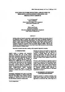
In this study, GPS/Gallieo measurements were simulated using the Matlab Toolboxes from GPSoft. The selected site was Sydney (Lat.33.53 degrees, Log. 151.10 degrees, height: 0.0m). The availability of GPS/Galileo satellites for the period of a wholly day is shown in Figures 1 and 2. If Gallieo constellation is included, there are at least 10 satellites available for navigation with a 15-degree masking angle. The measurement update rate was 1Hz and single frequency pseudorange measurements with standard deviation of 1 m. The simulated error sources include tropospheric error; multipath error; and ionospheric error, etc. There were 5 satellites from the GPS constellation: PRN4, PRN16, PRN18, PRN 19, PRN21 and 9 satellites from Galileo constellation: PRN202, PRN203, PRN204, PRN216, PRN217, PRN218, PRN224, PRN225, PRN226. These satellites were numbered from 1 to 14 for the convenience of discussions below.
4
Satellite Visibility 18
16
14
number of satellites
12
10
GPS+Galileo
8
6
4
2
0
0
5
10 Time of Day (hours)
15
20
Figure 1 Availability of GPS/Galileo Satellites
SATELLITE SKYPLOT NORTH
4 216 18225
226
204
224 19
21 WEST
EAST 217 203
218 16 202
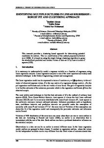
SOUTH Simulated GPS+GALLIEO Constellation
Figure 2 Status of the satellite constellation at the beginning of the simulation 3.2 Performance comparison between the LS and M-estimation schemes
Simulated data sets were added with a number of outliers. When there outliers of 10m were randomly added to the pseudorange observations over 1000 epochs, the navigation solutions are shown in Figs. 3, 4 and 5 blow.
5
10 0 -10 -20 -30
0
100
200
300
400
500
600
700
800
900
1000
0
100
200
300
400
500
600
700
800
900
1000
0
100
200
300
400
500
600
700
800
900
1000
20 0 -20 -40 5
0
-5
Figure 3 Estimated coordinates corrections for X,Y, Z (m) with three outliers using the LS 5
0
-5
0
100
200
300
400
500
600
700
800
900
1000
0
100
200
300
400
500
600
700
800
900
1000
0
100
200
300
400
500
600
700
800
900
1000
4 2 0 -2 -4 4 2 0 -2 -4
Figure 4 Estimated coordinates corrections for X,Y, Z (m) with three outliers using Huber
6
5
0
-5
0
100
200
300
400
500
600
700
800
900
1000
0
100
200
300
400
500
600
700
800
900
1000
0
100
200
300
400
500
600
700
800
900
1000
4 2 0 -2 -4 4 2 0 -2 -4
Figure 5 Estimated coordinates corrections for X,Y, Z (m) with three outliers using IGGIII
The results shown in Figures 3, 4 and 5 have clearly demonstrated the advantages of using Mestimation schemes over the traditional LS method. To further compare and investigate the potential performances of the LS and M-estimation schemes. More comprehensive computations have been conducted. The number of the simulated outliners varied from 1 to 7. Both the LS and M-estimation schemes were used to process the data sets. The results are presented in Tables 1-4. Table 1 Comparison between LS and M-estimation (with no or one outlier) Added outliers Sat. No. Estimation Schemes X (m) Y (m) Z (m) Number of zero weight observations
LS -1.06 1.54 0.81 null
Outlier free N/A HUBER -1.06 1.54 0.81 null
IGGIII -1.06 1.56 0.81 null
One Outlier PRN 19 with 10m outlier LS HUBER IGGIII -15.69 -0.36 -1.49 -26.59 1.26 1.66 0.19 0.33 1.04 null
null
PRN 19
Table 2 Comparison between LS and M-estimation (with 2 and 3 outliers) Added outliers Sat. No. Estimation Schemes X (m) Y (m) Z (m) Number of zero weight observations
Two Outliers PRN4,PRN16 with 10m outlier LS HUBER IGGIII -19.31 -1.97 -1.48 -24.97 2.40 1.86 2.30 1.59 1.10 null
null
PRN4,PRN16
Three Outliers PRN4,PRN16 ,PRN226 with 10m outlier LS HUBER IGGIII -19.34 -2.49 -1.44 -25.13 3.17 1.68 2.47 1.65 1.18 PRN4, PRN16 Null null PRN226
7
Table 3 Comparison between LS and M-estimation (with 4 and 5 outliers) Added outliers Sat. No. Estimation Schemes X (m) Y (m) Z (m) Number of zero weight observations
LS -19.05 -25.22 2.24 null
4 Outliers PRN4, PRN 19, PRN217 PRN226 with 10m outlier HUBER IGGIII 1.71 -1.78 3.05 1.45 -2.80 1.27 PRN4, PRN19 null PRN217, PRN226
5 Outliers PRN4, PRN 19, PRN21 PRN217, PRN226 with 10m outlier LS HUBER IGGIII -9.99 7.30 16.81 -28.79 -1.65 -6.98 -6.46 -7.30 -14.49 PRN18 null null PRN225
Table 4 Comparison between LS and M-estimation (with 6 and 7 outliers) Added outliers Sat. No. Estimation Schemes X (m) Y (m) Z (m) Number of zero weight observations
6 Outliers PRN4, PRN 19, PRN21, PRN217, PRN224,PRN226 with 10m outlier LS HUBER IGGIII -2.09 5.11 15.52 -35.75 -2.62 -8.77 -14.59 -7.56 -15.64 PRN18, null null PRN225
7 Outliers PRN4, PRN 19, PRN21, PRN204,PRN217, PRN224,PRN226 with 10m outlier LS HUBER IGGIII -17.64 -0.68 0.77 -25.75 1.81 -0.57 -4.58 -5.33 -10.24 PRN18, PRN203 null null PRN216, PRN225
As expected, in the scenario with no outliner, both LS and the M-estimation schemes have produced the same navigation solutions (see Table 1). As the number of the outliers increases, the navigation solutions based on the LS scheme are significantly biased, but the same time, both M-estimation schemes (Huber and IGGIII) have effectively mitigated the effect of these outliers (see Tables 1, 2, 3). It is noted that in Tables 3 and 4, when the number of the outliers reached 4 or higher, the navigation solutions based on both M-estimation schemes were somehow biased. This phenomenon indicates that the reliability of a robust estimation method to mitigate the multiple outliers is not without limit. The capacity of a specified M-estimation scheme should also be evaluated as part of the quality control procedure for the M-estimation methods. 4. Concluding Remarks
Over the next few years, multiple constellation satellite navigation systems will be developed, such as the modernized US GPS, Russian GLObal NAvigation Satellite Systems (Glonass), European satellite navigation system: Galileo, and, Chinese Compass (Beidou) Navigation Satellite System: CNSS (Gibbons, 2006). On the one hand, as the number of visible satellites is to be tripled or even more, the availability of the GNSS navigation services will be significantly improved. On the other hand, however, within the multi-constellation GNSS system, there will be an increased likelihood that multiple failures can occur. Therefore, a reliable procedure to mitigate the effect of the multiple outliers in the GNSS navigation solutions needs to be developed. Whilst, the current RAIM procedures are mainly based on the assumption of singe fault/outlier, the robust estimation theory can effectively address the multiple outlier scenarios. However, the comparison between the traditional RAIM procedure and the robust estimation methods should be further investigated using various data sets.
8
This paper has investigated the two M-estimation schemes, i.e., Huber and IGGIII, for use in mitigating the effect of outliers in the GNSS navigation solutions. The initial results from this study are promising. With the traditional RAIM methods, the outliers or faulty measurements are identified and the navigation solutions are statistically evaluated with the so-called protection levels. With the robust estimation methods, a new concept framework towards the GNSS integrity or the quality control of GNSS navigation solutions is required and should be further investigated. References
Baarda, W. (1968) A testing procedure for use in geodetic networks, Netherlands Geodetic Commision, New Series 2, No 4. Cross, P. A., Hawksbee, D. J. & Nicolai, R. (1994) Quality measures for differential GPS positioning, The Hydrographic Journal 72, 17–22. Förstner, W. (1983) Reliability and discernability of extended Gauss-Markov models, Deutsche Geodätische Kommission (DGK) Report A, No. 98, 79–103. Gibbons G. (2006) Compass: And China’s GNSS Makes Four. Inside GNSS, 1(8): 14. Hawkins D. (1980) Identification of Outliers, Chapman & Hall, London/New York. Hewitson S. and Wang J. (2006) GNSS Receiver Autonomous Integrity Monitoring (RAIM) for Multiple Outliers, European Journal of Navigation, Volume 4, Number 4, Sep 2006, Pages 47-54. Hewitson S., Lee H. K. and Wang J. (2004) ‘Localizability analysis for GPS/Galileo Receiver Autonomous Integrity Monitoring’, The Journal of Navigation Royal Institute of Navigation, 57, 245–259. Huber P. J. (1981) Robust Statistics, John Wiley, New York. Lee Y.C. (1986) Analysis of range and position comparison methods as a means to provide GPS integrity in the user receiver, US Institute of Navigation Annual Meeting, June 2426, 1-4. Miller K. M., Abbott V. J. and Capelin, K. (1997) ‘The reliability of quality measures in differential GPS’, The Hydrographic Journal 86, 27–31. Wang J. and Chen Y. (1999) ‘Outlier Detection and Reliability Measures for Singular Adjustment Models’, Geomatics Research Australasia, 71, 57-72. Xu P. L. (1993) Consequences of constant parameters and confidence intervals of robust estimation.Boll Geod Sc Aff 52:231-249. Yang Y., Cheng, M.K., Shum,C.K., and Tapley, B.D. ( 1999 ) Robust Estimation of systematic errors of satellite laser range Journal of Geodesy 73,345-349.
9