either white or black, and it is associated with a leaf (terminal) node of the ... other kind of quadtrees allows data to be stored only in leaves (terminal nodes).
J. King Saud Univ., Vol. 17, Comp. & Info. Sci., pp. 43-60 (A.H. 1425/2004)
ML-Quadtree: The Design of an Efficient Access Method for Spatial Database Systems A. Touir Department of Computer Science, College of Computer and Information Sciences King Saud University, Riyadh, Saudi Arabia (Received 28 April 2003; accepted for publication 4 October 2003) Abstract. The aim of this paper is to present a new indexing technique that provides an efficient support for retrieving and handling spatial data. Traditionally, the mapping between layers (in a thematic point of view) and index structures is one to one. Each layer is associated with an index structure. In some previous work, we have presented a data structure, the FI-Quadtree that handles a set of images using only one index structure. This handling is a raster-oriented format. In this paper, we focus on the processing of these objects from the vector oriented format point of view. The Multi-Layer Quadtree (ML-Quadtree) is a new data structure that allows the storage and processing of several layers at the same time. This structure is based on the PMQuadtree, which allows the storage of only a single-layer map. The aim of the ML-Quadtree is to be able to manage, store and perform queries among multiple layers simultaneously. The design and the manipulation of the proposed structure is presented in this paper whereas the implementation and the experimentation result will be treated in a subsequent paper.
1. Introduction Spatial Information systems require an efficient spatial data handling [1, 2]. The large amount of information and the complexity of the characteristics of data have given rise to new problems of storage and manipulation. One of the important problems is how to store this kind of complex data for efficient search and retrieval operations. Convenient data organization for spatial databases is still a problem to be solved [3, 4]. Data structures for storing objects in a vector format should satisfy various characteristics. In fact, there is a trade-off between retrieval capabilities and storage or memory requirement, and this is an important issue for spatial data handling. The organization of spatial data objects requires the ability to cluster them together according
43
A. Touir
44
to their spatial location. The number of required disk accesses is usually used to measure the efficiency of the operations. The first approach adopted in most reported research on spatial access methods considered that free-form objects could be approximated by their minimum bounding rectangles [5] to simplify the complexity of the search. R-trees [6] and their extensions R+trees [7], R*trees [8], and other structures such as buddy tree [9] are examples of such structures. Another approach is to consider the object as it is without any approximation. In this case, the space is subdivided according to certain rules. A commonly used data structure that fits this approach is the quadtree [10,11]. An other approach is to use the SP-GiST index structure [12]. This latter aims at partitioning unbalanced trees where it can behave as a quadtree, or any of its variants. Another similar approach [13], the GL/GiST were proposed to deal with spatial index based on granular locking technique. Quadtrees provide an interesting technique to code images either in a raster format or in a vector format. In this paper we will be dealing with the vector format using the quadtree approach. The quadtree is a hierarchical data structure used to organize an object space. An object can be a point, a line segment, a polyline, etc. This data structure has been widely used in computer vision, geographic information systems and geometric modelling [14]. Its main advantage is its compactness and regularity. Consider that we have a binary image; the principle of this structure consists in partitioning each object into homogeneous quadrants and labelling each of them. A homogeneous quadrant could be either white or black, and it is associated with a leaf (terminal) node of the quadtree. A non-homogeneous quadrant is considered as a grey quadrant and it is associated with a non-terminal node of the quadtree. Recursive subdivision is applied to the binary image: a quadrant is subdivided into four equal parts until a homogeneous quadrant or pixel is reached. The Morton order [15] can be used to organize and sort the squares that aggregate the space. Fig.1 shows how squares are ordered and labelled. 1
2
5
6
0000
3
4
7
8
01 00 0010 0011 0110 0111
9
10
13
14
1000 1001 1100 1101
11
12
15
16
1010
0001 0100 0101
11 10 1011 1110 1111
Fig. 1. Ordering squares using Morton order.
The Morton code of a node [16] is built by interleaving the bits of x and y coordinates of the upper left corner of the quadrant that corresponds to the node. The label of a quadrant, which we call a prefix, may have several representations. In this paper, we
ML-Quadtree: The Design of an Efficient Access . . .
45
suppose that a prefix can be defined either by its binary label, or by its length (number of bits that compose it) and its decimal value. The length of each binary label depends on the image definition. Within a 2N x 2N bitmap image, the maximum length is 2N. Some varieties of quadtrees have been proposed. Each one is more or less adapted to manipulate a specific type of data. Linear quadtrees are used to code and store black quadrants. The PM-Quadtree [11] represents line-segments data. Section 2.1 explains this structure in more detail. Hjaltason improved the bulk-loading PMR quadtrees [17,18]. Its principle consists in assuming that the quadtree is implemented using a linear quadtree, a disk-resident representation that stores objects contained in the leaf nodes of the quadtree is in a linear index ordered on the basis of a space-filling curve as shown above. The PR-Quadtree [19] is used to code point and region data. Another kind of quadtree is the MX-CIF-Quadtree [20]. It is used to represent data of type rectangle. The principle of the MX-CIF-Quadtree is to associate with each rectangle, the quadtree node corresponding to the smallest quadrant that contains it. The decomposition of quadrants is recursively carried out until no quadrant contains any rectangle. The last two types of quadtrees accept more than one data in a node. Moreover, using the MX-CIF-Quadtree, data can be in any node (root, terminal or non-terminal nodes), whereas the use of the other kind of quadtrees allows data to be stored only in leaves (terminal nodes). All the presented spatial structures allow the storage and indexing of a single object whatever this object is: a map, an image, etc. One quadtree is built for one object. On the contrary, the FI-Quadtree [21,22] allows the storage of a set of images into a single quadtree without any substantial difference from the complexity viewpoint. The DI-Quadtree [23] is an improved version of the FI-Quadtree. Its main differences with the FI-Quadtree reside in the labeling order of the nodes and in the storage mechanism. Given the number of layers, the FI-Quadtree computes in advance the necessary space needed to store them. If this number should be modified, the FI-Quadtree is reorganized to create more rooms for those additional layers. On the contrary, the DI-Quadtree is defined independently of the number of layers and it is used as a front structure. Both structures are raster-oriented. The MOF-tree [24] is also a raster–oriented structure. Its aim is to support images with multiple overlapping features. Its principle consists in recursive decomposition of the image into four equal-sized quadrants until each quadrant is fully covered by features covering it. Same is the case [25] with Multiversion Linear Quadtree, a spatio-temporal access method based on Multiversion B-trees [26]. The structure may be used as an index mechanism for storing and accessing evolving raster images. Unfortunately, all these quadtrees are not suitable when a given object, say a map, is composed of several layers where layers are in vector-oriented format. Layers are used for the purpose of thematic approach. Layers may represent districts, parcels, or a network of roads, rivers, etc., one layer per theme. Several index structures are used to
46
A. Touir
process queries like: "Retrieve all the water pipes and the electrical cables situated in a given region”. The use of a single index structure to perform such query is an attractive track. In this paper, we focus on this type of problem and show that our proposed data structure is suitable for this kind of queries. The use of the Multi-Layer-Quadtree (ML-Quadtree or MLQ for short) considerably reduces the complexity of the process of this type of queries in terms of I/O, time consumption and storage. Its flexibility resides in the fact that only one index structure is used to manage several layers. Another application of this structure is to manage multiple versions or temporal evolution of an object in a spatial databases context. The paper is organized as follows. In Section 2, we review the definition of the PM-Quadtree and introduce the Multi-Layer-Quadtree: its definition, characteristics, and properties. This section also deals with the proposed index structure. Section 3 gives some details of the multiple layers search within the proposed structure; it introduces the principle of the Insert and Delete operations and discusses the capabilities provided by the ML-Quadtree in querying several layers. Finally, conclusions are given in Section 4. 2. The Multi-Layer-Quadtree Data Structure 2.1 Principles of the PM-Quadtree The PM-Quadtree (PMQ) [11] represents objects of polygonal shapes. The representation of objects is neither approximated nor based on digitization. Different kinds of arithmetic and geometric operations could be performed using this type of structure without any distortions of the objects. This is in contrast with the bitmap/raster representation, where zooming in on, or rotating, an object may change its original shape. In addition, the PMQ allows each entity of the stored object to have a semantic meaning such as lake, hotel, road, etc. Different kinds of PM-Quadtrees are used. Each of these PMQs consists in subdividing each region into four equal-sized quadrants until we obtain quadrants that satisfy the following rules [12]: PM1-Quadtree (Fig.2.a): At most, one polygon vertex can lie in a region represented by a quadtree leaf node. If a quadtree leaf node region contains a vertex, then any edge of this region must contain that vertex. If a quadtree leaf node region does not contain vertices, it can contain at most one edge. Each region quadtree leaf node is maximal and contains at most one vertex. PM2-Quadtree (Fig.2.b): It differs from PM1-Quadtree in that a region is decomposed into four equal-sized quadrants as long as a quadrant contains more than one line segment unless the line segments are all incident to the same vertex.
ML-Quadtree: The Design of an Efficient Access . . .
47
PM3-Quadtree (Fig.2.c): The decomposition depends only on the vertices. A region is decomposed into four equal-sized quadrants as long as it contains more than one vertex. Bucket PM-Quadtree (Fig.2.d): Recursively decomposes a region into four equal-sized quadrants as long as a quadrant contains more than BC line segments. BC is called the bucket capacity of the PM-Quadtree. Table 1 reflects the prefixes and the data generated from each kind of PM-Quadtree shown in Fig. 2.
B
D
B
F
D
E
E
A
A
C
(a) PM1Quadtree
B
D
B
E
D
F E
A
C
c) PM3-Quadtree
C
(b)PM2-Quadtree
F
A
F
C
d)- Bucket PM-Quadtree with BC = 2
i. Fig. 2. Principle of subdividing the space using different PM-Quadtrees.
A. Touir
48
Table 1. List of prefixes and their related data generated from the example of Fig. 2 according to the type of PMQ used Quadtree type
List of prefixes and their related data
PM1Q
{(0000, B),(0001, D),(001000, AB),(001001, BC),(001010, AB),(001100, BC),(001101, DE), (001110, BC),(001111, BC),(0101, F),(0110, E),(0111, EF),(1000, A),(1001, BC),(11, C)}
PM2Q
{(0000, B),(0001, D),(0010, [AB, BC]),(001100, BC),(001101, DE), (001110, BC),(001111, BC),(0101, F),(0110, E),(0111, EF), (1000, A),(1001, BC),(11, C)}
PM3Q
{(0000, B),(0001, D),(0010, [AB, BC]),(0011, [BC,DE]) ,(0101, F),(0110, E), (0111, EF), (10,A),(11,C)}
Bucket-PMQ
{(0000, B),(0001, D),(0010, [AB, BC]),(0011, [BC,DE]),(01, [E,F]), (10,A), (11,C)}
As we can notice, with the same data, a generated PMQ is more or less complex depending on its definition (i.e. the number of items that could be contained in a quadrant). PM1Q generates much more nodes than the other PMQs. A PM1Q leaf node contains no more than one item (a vertex or a line segment). On the contrary, the other PM-Quadtrees allow a leaf node to contain several items and, so, they need additional processing. 2.2 Basic Idea We consider a layer as a set of spatial objects and a map as a set of layers. A spatial object may be part of several layers. In addition, queries may trigger the processing of several layers, in search for the requested spatial objects. This multi-layer processing is a complex operation. This complexity is due to the fact that the data set of the spatial objects is very large. It is, therefore, crucial to support indexing techniques to facilitate the retrieval of any portion of an object. In order to overcome this problem, we present a Multi-Layer-Quadtree that allows for the processing of components of different layers in the same structure. This processing could be considered as a multiple join operations or a multiple criteria selection. We define MLQ as being based on the PM1Quadtree. This choice of PM1Quadtree is due to the fact that the number of nodes of the MLQ grows with respect to the inserted layers. So, nodes that are not generated from one layer may be generated from others. As indicated, earlier, all PMQs but PM1Q need additional processing to determine the right vertices; for this reason, we have chosen PM1Q as the basic structure for the MLQ to avoid the extra processing. Applying the MLQ based on the other PMQs may be presented as future work. 2.3 The Multi-Layer-Quadtree: Definition and Characteristics
ML-Quadtree: The Design of an Efficient Access . . .
49
Similar to the DI-Quadtree, the ML-Quadtree is defined as a pure index structure, where each node is a pointer to a structure that contains the data belonging to that node (Fig. 3). The maximum number of nodes that constitute an MLQ is
�
4 N �1 �1 3
nodes. For
N = 10 we have a total of 1398101 nodes. The fact that the MLQ is used as a pure index structure allows us to manipulate it as a main memory-oriented structure. Each node addresses a rear structure defined as follows: x x
Each rear structure is composed of a set of components {c1, …, ck}. Each component ci is defined as being a triplet (layeri, objectj, elementk), where elementk (e.g. a line) belongs to objectj (e.g. a polyline), which in turn belongs to layeri. As it is described in [23], after several insertions in a given rear structure (say RS), the latter may be full; in which case a new rear structure is created and logically linked to RS. Figure 3 shows how a new layer is inserted and handled with the ML-Quadtree and its rear structure.
x x
MLQ
G
E J D
�����H
�����D
�����J
�����GH
�����G
�����E
(a)
�����JG
H
(b) Fig. 3. Inserting a first layer in the ML-Quadtree.
Table 2. List of symbols and definitions Symbol
Definition
N QN PN WN HN q. p Lp Vp b
Number of decompositions of the ML-Quadtree Workspace of size 2Nx2N, consisting of all quadrants of a 2 Nx2N image The set of prefixes associated with QN A set of integers defined as: WN={w/ �pPN,w=HN(p)} A mapping function between PN and WN A quadrant of QN An element of PN associated with a quadrant q The number of bits that compose p The decimal value of p Bit value
RS
A. Touir
50 w Lmax Scap
A node value. w belongs to WN The maximum number of layers in the MLQ The maximum number of components that can fit in a segment of the rear structure
We denote nd=(w, {c1, …, ck}) a node of an ML-Quadtree, where w is a node label and {c1, …, ck} is the set of components indexed from that node. A triplet (Li, Oj, Ek) defines a component ci, where Ek is the element of the object Oj belonging to the layer Li. An ML-Quadtree is a quaternary tree that satisfies the following: i) Data of an ML-Quadtree is indexed from any node. Three components c1, c2, c3 could be distributed on three nodes nd1, nd2, nd3 of three different levels, where nd1=(w1,{c1}) is a parent of nd2=(w2,{c2}), which is in turn a parent of nd3=(w3,{c3}). ii) if (w�,{c1, …, cn}) and (w�, {d1, …, dm}) are in the same path, ci and dj could not belong to the same layer, for any i= 1, ..., n and j = 1, ..., m; i.e two components of the same layer must not be in the same path unless they are in the same node. iii) The Morton code is used to label the upper left corner of the quadrant that corresponds to a node. In this paper, we suppose that a prefix can be defined either by its binary representation p, or by its length Lp (number of bits that compose it) and its decimal value Lp
Vp
¦b * 2
( Lp �i )
i
. Thus for any prefix p = b1b2b3…bLp= (Lp, Vp),
i 1
where
bi {0,1} .
In the sequel and by notation abuse, we use any of the two representation (p or (Lp,Vp)). As defined in (Touir, 1991),
H N ( p)
where
:
Lp 2
Lp
� ¦ bi * : i , i 1
�1 °4 if i is even . ® °2 * :3 if i is odd i �1 ¯ i ( N � �1) 2
This function offers a total order of labeling between P N and WN. It reflects a pre-order traversal of the ML-Quadtree (Fig. 4). Note that HN is a 1-1 onto mapping. Thus, it could be used to index nodes in a unique way.
ML-Quadtree: The Design of an Efficient Access . . .
51
Suppose that we have already inserted a layer (say X) represented in Fig. 3, and we would like to insert a new one (say Y) represented in Fig. 5. By applying the above defined rules (i-iv), we obtain a virtual layer (say Z) Z=XY (Fig. 6). Z is the superimposition of X and Y. 0
40
23
1
43
2
7
22
12 17
23
28
33 38
39
(a)
43
40
44 49
64
54 59
65
70
75 80
41 42
(b)
Fig.4. The labelling of quadrants in a quadtree (decimal values-pre-order traversal).
&
'
&
%
( $
(a)
)
' % %$
$
(
)
(b) Fig. 5. Building a second layer component.
By applying (i), we see that Z has components distributed on many levels: (2,1,') is a component in a node of level 1. This node is a parent of {(1,1,JG), (1,1,G), (1,1,J), (1,1,GH)}. By applying (ii), we see that if a component of X (resp. Y) is in a given node, all its subnodes (children) do not contain any component of X (resp. Y).
A. Touir
52
G E
J
' &
( %
D
�����)
�����(
Fig. 6. How the ML-Quadtree changes when a new layer is inserted.
�����H � �����D �����$
�����$% �����%
�����'
�����J
�����GH
�����G �����JG �����E ������&
(b) (a)
H
) $
ML-Quadtree: The Design of an Efficient Access . . .
2.4 Indexing Technique As it was mentioned, the maximum number of nodes of an MLQ is
53
�
4 N �1 �1 3
nodes. We intend to use the MLQ as a pure main memory oriented index structure. For this reason, we choose an index whose size is small enough to give the needed information and to keep the MLQ reasonably small so that it can fit in the main memory. As an illustration, consider the MLQ in Figure 4.a, where N=3, q1, q2 and q3 three quadrant regions, then their corresponding prefixes are respectively p 1=10=(2,2), p2=0100=(4,4) and p3=011101=(6,29); Using HN and :i where i=1…6, we obtain: w1= HN (p1)= 1+:1= 43, w2 = HN (p2)= 2+:2= 23 and w3 = HN (p3) = 3+:2+:3+:4+:6= 40. By the definition of w and p, it can be seen that the size of w is smaller than the size of p. Consequently using w as an index will reduce considerably the size of MLQ. To use w -1
as an index, we need to introduce the notion of HN , which is the inverse of HN. We -1
-1
denote HN with GN (i.e. GN=HN ). The intention is to determine pPN for every w in WN. That is �wWN, �pPN / p=GN(w). With this in mind, we have developed the algorithm below to compute p PN / p= GN(w) for each given wWN: G N:
input : w a value that belongs to WN, N output : p a value that belongs to PN length_of_p = 0 value_of_p = 0 for i=2N downto 1 do if w> :2N-i+1 then value_of_p = value_of_p0 then value_of_p = value_of_p