MLP-BASED SOURCE SEPARATION FOR MLP ... - Semantic Scholar

4th International Symposium on Independent Component Analysis and Blind Signal Separation (ICA2003), April 2003, Nara, Japan

MLP-BASED SOURCE SEPARATION FOR MLP-LIKE NONLINEAR MIXTURES R. Mart´ın-Clemente♦ , S. Hornillo-Mellado♦ , J. I. Acha♦ , F. Rojas† , C. G. Puntonet† ♦´

Area de Teor´ıa de la Se˜ nal y Comunicaciones, † Dpto. de Arquit. y Tecnol. de Computadores Universities of Sevilla♦ and Granada† — (SPAIN) E-mails: {ruben,susanah,acha}@us.es, {frojas,carlos}@atc.ugr.es ABSTRACT

1.1. Nonlinear BSS: a short review The problem of nonlinear mixtures is that separation is impossible without additional prior knowledge of the mixing model, as the independence assumption is not strong enough [10, 19]. In practice, special nonlinear mixing models are assumed in order to simplify the problem: for example, consider Wiener and Hammerstein models (see [4], chapter 12 and [20]) and the post-nonlinear mixture case [19]. In addition, Deco and Brauer [5] have addressed the problem by considering that the mixing mapping satisfies a volume conserving condition, which ensures that it is invertible. Hyv¨ arinen and Pajunen [10] have shown that, in the twosource case, separation is feasible if the mixing function is a conformal mapping. Several algorithms and methods show promise in the nonlinear BSS problem. To our knowledge, the first solution was given by Burel [2], who proposed a neural network to minimize the energy of the difference between the joint probability density function (pdf ) and the marginal pdfs of the estimated sources. Almeida [1] and Koutras et al [16] have addressed the problem using a nework with an adaptable nonlinearity as separating system. They claim that it shows a great flexibility towards fitting complex nonlinear mixing functions. Radial Basis Functions have also been employed as separating system: specifically, good results have been reported by Tan et al [21]. Locally linear BSS methods have been recently explored by Karhunen et al [15] using a K-means-clustering-based method. Pajunen et al (see [9], Chapter 17 and the references therein) use Kohonen’s self-organizing-feature maps (SOFM). Their approach holds when the sources have pdfs with bounded supports. See also [14] and the references therein. One of the greatest problems encountered in nonlinear source separation is that algorithms that are based on a gradient-descent adaptation are often trapped within local minima. For this reason, Puntonet et al [17] use simulated annealing to avoid undesired minima in the training of a modified Kohonen’s network. In addition, Rojas et al [18] propose a separating system which approximates the nonlinearities of the post-nonlinear mixture model by means of odd polynomials and makes use of genetic algorithms for the optimization of the system. The post-nonlinear case is also dealt by Taleb and Jutten [19], who propose to minimize the mutual information between the estimated sources using a nonlinear system

In this paper, the nonlinear blind source separation problem is addressed by using a multilayer perceptron (MLP) as separating system, which is justified in the universal approximation property of MLP networks. An adaptive learning algorithm for a perceptron with two hidden-layers is presented. The algorithm minimizes the mutual information between the outputs of the MLP. The performance of the proposed method is illustrated by some experiments.

1. INTRODUCTION. Blind Source Separation (BSS) is a fundamental problem in signal processing. It consists of retrieving unobserved sources s1 (t), . . ., sN (t), assumed to be statistically independent (which is phisically plausible when the sources have different origins), from only M observed signals x1 (t), . . ., xM (t) which are unknown functions or mixtures of the sources. In general, samples of each source are not assumed to be independent and identically distributed (i.i.d) and no assumption concerning the temporal dependence between them is used. In this paper, we restrict the study to the case N = M , where the number of sources is equal to the number of sensors. Starting from the seminal work [12, 13], this problem has been intensively studied over the last decade and there exist elegant solutions when the mixtures are linear and instantaneous (see [4, 6, 9] and the references therein). If the mixture is nonlinear, on the contrary, few algorithms have been presented and they are not completely effective. In this paper, the latter problem is addressed by using a multilayer perceptron (MLP) as separating system, which is justified in the universal approximation property of MLP networks [7]. An adaptive learning algorithm for minimizing the mutual information between the outputs of a perceptron with two hidden-layers is presented. The performance of the proposed method is then illustrated by some experiments. The paper also introduces the problems of using MLPs with more-than-one hidden layer in the context of BSS.

155

that precedes a linear separating stage. The nonlinear mapping from the observations to the sources can also be modeled using multilayer perceptrons (MLP). Yang et al [22] use a two-layer perceptron as system to separate the sources. They ensure that the neural network is invertible by setting the number of neurons in the hidden layer to the number of sources. This is a very severe constraint that endangers the approximation capabilities of the net. Nevertheless, if such a constraint is eliminated (as, for example, in the ensemble learning approach [14]), one meets serious mathematical dificulties and a high computational complexity. Hence, rather than increasing the number of neurons in the first hidden layer, the solution may be the use of two of more hidden layers. In Sections 2 and 3, this basic idea is developed into a practical proposal. In Section 4, learning rules for the MLP are derived. Section 5 contains the results of experiments conducted to show the performance and potential problems. Section 6 contains our main conclusions.

W3

u(t)

z(t)

f

v(t)

g

W2

y(t)

W1

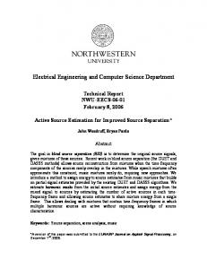
Figure 1: Neural Network Arquitecture.

3. CRITERION FUNCTION 3.1. Information-Theoretic Criterion The guiding principle of unsupervised source separation is, in most approaches, to transform the observed data so that the transformed variables are as mutually independent as possible. Even thought that this transformation is not unique in the non-linear mixture case, numerous experiments show that one often separates the sources (see, for example, [16, 21, 22]). In explanation of this favourable behaviour, one can conjecture that separating systems with few parameters (i.e., degrees of freedom) work because they are not able to produce signals that are more independent than the original sources, provided that the nonlinear mixture of the sources was smooth and can be undone through a smooth transformation. The conjecture seems to be valid for a wide range of source pdfs. The degree of dependence between the outputs is commonly quantified by their mutual information, which is defined as: N X I(y) = −H(y) + H(yi ) (3)

2. MODEL STRUCTURE Let s(t) = [s1 (t), . . . , sN (t)]T with si (t), i = 1, . . . , N being N mutually independent random processes whose pdfs are unknown. Suppose that we have N sensors; the output of each one denoted by xi (t), i = 1, . . . , N , which measure a combination of the N sources. In a vector form, this is expressed as x(t) = F(s(t)) (1)

i=1

where x(t) = [x1 (t), . . . , xN (t)]T is called the observation vector, being the information that is available, and F : RN → RN is an unknown memoryless differentiable bijective (reversible) mapping. The task of BSS is that of recovering the sources from the observed signals. Here, the idea is to approximate the inverse of F by using the neural network shown in Figure 1, as MLPs have the universal approximation property for smooth continuous mappings. Such a network is described by the equations: F −1 (x(t)) ≈ y(t) = W1 g(u(t) + b1 )

w(t)

x(t)

where H(· ) is the Shannon differential entropy. A wellknown property is that I(y) ≥ 0 with equality if and only if the outputs are independent. For the sake of simplicity, other measures of independence (such as, for example, that given in [2] or Renyi’s mutual information [8]) have not been taken into account. 3.2. Practical Cost Function By using (2), −H(y) can be easily expanded as:

(2a)

−H(y) = −H(x) −

3 X

log | Wi | −

i=1

being u(t) = W2 f (w(t) + b2 )

−

(2b)

N X

E[ log | gi0 (ui + b1i ) | ] −

i=1

and w(t) = W3 x(t)

N X

E[ log | fi0 (wi + b2i ) | ] (4)

i=1

where H(x) is the joint entropy of the observed signals,

(2c)

| Wi |=| det(Wi ) |,

where W1 , W2 and W3 are square matrices,

bji stands for the i-th component of vector bj and gi0 (· ), fi0 (· ) are the first-order derivatives of gi (· ) and fi (· ), respectively. Since the term H(x) in expression (4) does not depend on the parameters of the MLP, the minimization of the mutual information between the outputs is equivalent to minimize the index:

g(vector) = [g1 (vector1 ), . . . , gN (vectorN )]T , f (vector) = [f1 (vector1 ), . . . , fN (vectorN )]T , where vector = [vector1 , . . . , vectorN ]T , gi (· ) and fi (· ) are any continuous sigmoid-type function and both b1 and b2 are N × 1 vectors. Since the mixing system is memoryless, notice that we will drop time index t in the following.

def

I(y) = I(y) + H(x)

(5)

One serious problem is that the exact calculation of the marginal entropies H(yi ) is rather involved. If we assume

156

that the outputs are standardized (i.e., they are zero-mean unit-variance signals), their entropies can be approximated as (see [9], chapter 5 and [22]): H(yi ) ≈

since ui =

X

the skewness measure of yi and = kurtosis. In order to encourage such a standardization, Tikhonov regularization terms are added to (5) according to J (y) = I(y) + λ1

2

(E[yi ]) + λ2

i=1

N X

N X

3 wjq xq + b2j )

i

X gi00 2 0 ∂ log | gi0 |= wik fk xp 3 ∂wkp gi0 i

− 1)

2

(15)

where fk0 is the first order derivative of fk . Hence, by setting def

(E[yi2 ]

(14)

q=1

it follows that

κi4

N X

2 wij fj (

j=1

(κi )2 (κi )2 3 (κi )3 1 log(2πe)− 3 − 4 + (κi3 )2 κi4 + 4 (6) 2 12 48 8 16

where κi3 = E[(yi )3 ] is E[(yi )4 ] − 3 equals its

N X

0 Df (w) = diag(f10 (w1 + b21 ), . . . , fN (wN + b2N ))

(7)

it can be written that X ∂ log | gi0 |= −Df (w) WT2 Φg (u) xT ∂W 3 i

i=1

Using (4) and (6) in (7), J (y) can be estimated and minimized. We may impose some additional constraints or prior information on the sources (e.g. sparsity, super-gaussianity, and so on). Even though that the MLP may create sparse or super-gaussian outputs that do not recreate the original sources, Tan et al [21] have reported good results by imposing perfect matching of moments between the outputs of the net and the sources. In addition, we are conscious of the asymmetry of the cost function, since H(y) is exactly calculated whereas the marginal entropies H(yi ) are only approximated by using a Gram-Charlier expansion (which, in addition, assumes that the pdfs are not very far from the Gaussian density). Both problems should be addressed in future investigations.

Similarly, wi =

X

3 xj wij

(16)

(17)

(18)

j

thus,

X i

f 00 ∂ 0 (wi + b2i ) |= k0 xp 3 log | fi ∂wkp fk

(19)

and, consequently, X i

∂ log | fi0 (wi + b2i ) |= −Φ(w) xT ∂W3

(20)

where def

Φf [w] = −[

4. LEARNING RULES In the following, let bji denote the i-th entry of vector bj . k Similarly, wqp will stand for the (q, p)-th component of matrix Wk .

00 f100 (w1 + b21 ) fN (wN + b2N ) T ] 0 2 ,..., 0 f1 (w1 + b1 ) fN (wN + b2N )

(21)

Finally, we obtain ∂H[y] ∂W3

= W3−T − E[Df (w) W2T Φg (u) xT + Φf (w) xT ] (22)

4.1. Differentiating the joint entropy H(y)

and, similarly

It is well-known that ∂ log | Wi | = W−T i ∂Wi

∂H[y] ∂b2

(8)

= −E[Df (w) W2T Φg (u) + Φf (w) ]

(23)

4.2. Differentiating the marginal entropies H(yi )

hence, ∂H[y] ∂W1

=

W−T 1

Using (6), some algebra shows that

(9)

∂H(yi ) ∂yi = E[yˆi ] ∂α ∂α

Similarly, we easily obtain ∂H[y] ∂W2

=

W−T 2

− E[Φg [u]zT ]

(10)

where

where def

Φg [u] = −[

00 gN g100 (u1 + b11 ) (uN + b1N ) T ] 0 1 ,..., 0 g1 (u1 + b1 ) gN (uN + b1N )

yˆi = {− (11)

= −E[Φg [u]]

(12)

k

Now, observe that ∂ g 00 ∂ui log | gi0 (ui + b1i ) |= i0 3 3 ∂wkp gi ∂wkp

3 3 1 κi3 9 i i 2 + κ3 κ4 }yi +{ (κi4 )2 + (κi3 )2 − κi4 } yi3 (25) 2 4 4 2 6

being κi3 = E[(yi )3 ] and κi4 == E[(yi )4 ] − 3. Hence, when 1 α = wij ∂ X H(yk ) = E[ˆ yi vj ] (26) 1 ∂wij

and ∂H[y] ∂b1

(24)

and, consequently (13)

∂ ∂W1

157

PN k=1

H(yk ) = E[ˆ y vT ]

(27)

2 ˆ = [yˆ1 , . . . , yˆN ]T . Secondly, when α = wij where y and using that ∂yk 1 0 (28) 2 = wki gi zj ∂wij

4.4. Natural gradient Finally, to avoid inverse matrix operations, we use the natural gradient rule (see [6], chapter 1) and derive the learning algorithm that appears in Table 1, i.e., the unsupervised learning rule for minimizing the mutual information between the outputs of a perceptron with two hidden layers. It is worth noticing that similar rules can be obtained by maximizing the entropy of these outputs instead of minimizing their mutual information.

we obtain X ∂ X 1 H(yk ) = E[ˆ yk wki gi0 zj ] 2 ∂wij k

(29)

k

Thus, it follows that P

∂ ∂W2

ˆ zT ] H(yk ) = E[Dg WT1 y

k

(30)

where def

Dg (u) =

diag(g10 (u1

+

0 (uN b11 ), . . . , gN

+

b1N ))

(31)

1.

d W1 dt

= {I − E[ˆ yyT ]}W1

2.

d W2 dt

ˆ uT ]}W2 = {I − E[Φg uT − Dg WT1 y

3.

d W3 dt

= {I − E[Df WT2 Φg wT + Φf wT + ˆ wT ]}W3 +Df WT2 Dg WT1 y

4.

d b dt 1

Using a similar procedure, it can be obtained that ∂ ∂b1

P k

ˆ] H(yk ) = E[Dg WT1 y

(32)

ˆ] = −E[Φg + Dg WT1 y

d ˆ] 5. dt b2 = −E[Df WT2 Φg + Φf + Df WT2 Dg WT1 y

The most involved calculation is the following one: since X 1 yk = wkp gp (up + b1p ) (33)

Table 1: Learning Rules.

p

and

∂up 2 0 3 = wpi fi xj ∂wij

(34)

5. COMPUTER SIMULATIONS

we obtain that XX ∂ X 1 2 H(yk ) = E[ˆ yk wkp gp0 wpi fi0 xj ] 3 ∂wij p k

In order to check the validity and performance of the proposed adaptive learning algorithm, it has been extensively simulated on a computer. Due to limited space, we shall present in this paper only a few illustrative examples. In all of them, we have employed a batch version of the learning algorithm (block size and learning rate were set to 100 samples and 0.001 respectively) and both regularization parameters λ1 and λ2 were set to 10. A little momentum term was also added to speed up the learning process.

(35)

k

or, in matrix form, ∂ ∂W3

P k

ˆ xT ] H(yk ) = E[Df WT2 Dg WT1 y

(36)

Similarly, ∂ ∂b2

P k

H(yk ) =

E[Df WT2

ˆ] Dg WT1 y

5.1. Experiment 1. Post-nonlinear mixture of two sources.

(37)

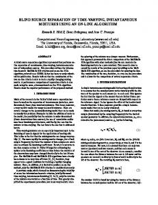
A simple experiment in which the net separates a postnonlinear mixture of two signals. All the signals are depicted in Figure 2. The mixtures were generated using the model: x = tanh(A s),

4.3. Taking Tikhonov regularization terms into account Tikhonov terms are X X λ1 (E[yi ])2 + λ2 (E[yi2 ] − 1)2 i

where (38)

i

0.3382 −0.1091

0.4768 0.6422



Separation is clearly achieved. In fact, separation is always possible under mild conditions [10] in the two-source case.

which is similar to (6) in the sense that both are a combination of statistics. Hence, the derivatives of the Tikhonov terms can be easily taking into account by incorporating ˆ: the following terms into the definition of vector y ˆ←y ˆ + 2 λ1 E[y] + 4 λ2 E[y ¯ y − 1] ¯ y y

 A=

5.2. Experiment 2.- “Hard” non-linear mixture of three sources.

(39)

In this case, the mixtures were generated as:

where ¯ stands for the Hadamard product and 1 is a vector of ones.

x = A1 tanh(A2 s),

158

ORIGINAL SOURCES

ORIGINAL SOURCES

OBSERVED (MIXED) SIGNALS

NONLINEAR MIXTURES

ESTIMATED SOURCES

ESTIMATED SOURCES

Figure 2: From the top to the bottom: sources, postnonlinear mixtures and estimated sources after 10 sweeps. Figure 3: From the left to the right, a) source signals b) nonlinear mixtures c) estimated sources (after 20 sweeps). where



−0.0882 A1 =  −0.2947 −0.7857 and



−0.7207 A2 =  −0.2900 0.8585

−0.1747 −0.7114 0.2968 0.8083 0.6680 0.9536

 −0.6919 −0.8542  , −0.7538

both W1 and W2 are often close to permutation matrices in the vicinity of the local minima.

 −0.4853 0.5059  −0.0655

6. DISCUSSION AND FUTURE RESEARCH The neural network has been applied to the nonlinear BSS problem. Our experiments mainly show that:

The mixing function is strongly nonlinear: it is noteworthy that the popular algorithm JADE ( [3], available at [11]) which was originally devised for linear mixtures, is not able to separate the sources. A 1000-sample training set was used for adjusting the network. In this experiment, the algorithm converges in about 20 sweeps. It has been found experimentally that matrices W1 and W2 adapt at a much slower pace than matrix W3 . Results are depicted in Figure 3 (only 80 samples of each signal are plotted for the sake of clarity). The estimation of the first and second sources seems to be acceptable. On the contrary, the third source is still distorted after separation. Figure 4 shows the magnitude of the Fourier Transforms of the third source and its estimate. Two interfering peaks which are caused by the other sources are clearly visible and we can easily realize that they are not harmonic components of the Fourier Transforms. Hence, it makes good sense to remove them in a post-processing stage even if we do not know that the three sources are periodic signals.

• In this context, networks with two hidden layers are more prone to fall into bad local minima than networks with a single hidden layer [22]. To avoid such undesired minima, we are currently investigating metaheuristics and global search methods1 . Promising results have been obtained by using an evolutionary algorithm [18]. Further research in this field would be clearly fruitful. • Separation is hindered by the fact that independencebased cost functions, such as (7), can not distinguish between the estimated sources y1 , y2 and y3 and any of their functions h1 (y1 ), h2 (y1 ) and h3 (y1 ), provided that y1 , y2 and y3 are mutually independent. 7. REFERENCES [1] L. B. Almeida, ”ICA of Linear and Nonlinear Mixtures Based on Mutual Information”, Proc. of International Joint Conference on Neural Networks (IJCNN 2001), available at http://www.cnel.ufl.edu/info/infopapers.html.

5.3. Experiment 3.- Local minima. This experiment demonstrates the existence of spurious local minima. We consider a nonlinear mixture of five uniform sources in which, according to our calculations, the minimum value of J (y) is about 10. Each learning curve in Figure 5 corresponds to different initial conditions. Separation is achieved in the experiment that corresponds to the bottom curve. It is noteworthy that

[2] G. Burel, “Blind Separation of Sources – A nonlinear neural algorithm”, Neural Networks, vol. 5, No. 6, pp 937-947, 1992. 1 The Genetic Optimization Toolbox was used, available at www.mathtools.net.

159

400

20

350

Interference due to the first source

Solid Line: Spectrum of the Original 3rd. Source

300 Dashed Line: Spectrum of the Estimated 3rd. Source

Cost Function

250

200

15

150 Interference due to the second source

10 100

50

0

0

0.05

0.1

0.15

0.2 0.25 0.3 Digital Frequency

0.35

0.4

0.45

5

0.5

(ω)

Figure 4: Fourier Transforms of the original and estimated source.

750

800

850

900 Iteration

950

1000

1050

Figure 5: Learning curves for different initial conditions. Only the curve plotted at the bottom of the figure corresponds to a successful separation.

[3] J-F. Cardoso and A. Souloumiac, “ Blind Beamforming for non-Gaussian Signals ”, Proceedings of the Inst. Elect. Eng., Vol.140 (F6), pp.362-370, 1993.

[14] J. Karhunen, ”Nonlinear Independent Component Analysis”. Everson and S. Roberts (Eds.), ”ICA: Principles and Practice”, pp. 113-134 Cambridge University Press, 2001. (available at: http://www.cis.hut.fi/juha/papers/nica-chap.ps.gz)

[4] A. Cichocki, S.I.Amari, “Adaptive Blind Signal and Image Processing”, John Willey and Sons, 2002. [5] G. Deco and W. Brauer, “Nonlinear higher-order statistical decorrelation by volume-conserving architectures”, Neural Networks, vol. 8, pp. 525-535, 1995.

[15] J. Karhunen, S. Malaroiu and M. Ilmoniemi, ”Local linear ICA based on clustering”, International Journal of Neural Systems, vol. 10, no. 6, pp. 439-451, 2000.

[6] S. Haykin, Ed., “Unsupervised Adaptive Fitering. Volume I: Blind Source Separation”, John Willey and Sons, 2000.

[16] A. Koutras, E. Dermatas and G. Kokkinakis, ”Neural Network Based Blind Source Separation of Non-Linear Mixtures”, Proc. ICANN, pp. 561-567, Vienna, Austria, 2001.

[7] S. Haykin, “Neural Networks – A comprehensive Foundation”, Prentice-Hall, 1998.

[17] C. G. Puntonet, A. Mansour, C. Bauer and E. Lang, “Separation of Sources using Simulated Annealing and Competitive Learning”, Neurocomputing (to appear).

[8] K.E. Hild II, D. Erdogmus, J.C. Pr´ıncipe, “Blind Source Separation Using Renyi’s Mutual Information”, IEEE Signal Processing Letters, vol. 8, no. 6, pp. 174-176, 2001.

[18] F. Rojas, I. Rojas, R. Mart´ın-Clemente and C.G.Puntonet, “Nonlinear Blind Source Separation using Genetic Algorithms”, Proc. ICA 2001, pp.771-774, San Diego, USA, 2001

arinen, J. Karhunen and E. Oja, “Independent [9] A. Hyv¨ Component Analysis”, John Willey and Sons, 2001.

[19] A. Taleb and C. Jutten “ Source Separation in PostNonlinear Mixtures ” IEEE Trans. on Signal Proc., Vol. 47, No. 10, pp.2807-2820, 1999.

arinen and P. Pajunen, “Nonlinear Indepen[10] A. Hyv¨ dent Component Analysis: Existence and uniqueness results”, Neural Networks, vol. 12, No. 3, pp 429-439, 1999.

[20] A. Taleb, J. Sol and C. Jutten “ Blind Inversion of Wiener Systems ” Proc. IWANN 99, pp.655-664, 1999

[11] http://sig.enst.fr:80/∼cardoso/stuff.html

[21] Y. Tan, J. Wang and J.Zurada, “ Nonlinear Blind Source Separation using a Radial Basis Function Network ” IEEE Trans. on Neural Networks., Vol. 12, No. 1, pp.124-134, 2001.

”Blind Separation of [12] C. Jutten and J. Herault, Sources, Part I: an adaptive algorithm based on neuromimetic architecture”, Signal Processing, vol. 24, pp.1-10, 1991.

[22] H.H. Yang, S.Amari and A. Cichocki, “InformationTheoretic Approach to Blind Separation of Sources in Non-Linear mixture”, in Signal Processing, vol. 64, No. 3, pp. 291-300, 1998.

[13] C. Jutten and A. Taleb, ”Source Separation: from dusk till dawn.”, Proc. 2nd. Int. Workshop on Independent Component Analysis and Blind Source Separation, pp. 15-26, Helsinki, Finland, 2000.

160