Abstract. In this paper we introduce a new technique for blind source separation of speech signals. We focused on the temporal structure of signals which.
An Approach to Blind Source Separation of Speech Signals Shiro Ikeda, Noboru Murata RIKEN Brain Science Institute Wako, Japan
Abstract In this paper we introduce a new technique for blind source separation of speech signals. We focused on the temporal structure of signals which is not always the case in other major approaches. The idea is to apply the decorrelation method proposed by Molgedey and Schuster in timefrequency domain. We show some results of experiments with artificial data and speech data recorded in the real environment. Our algorithm needs considerably straightforward calculation and includes only a few parameters to be tuned.
1
Introduction
In this paper, we propose a blind source separation (BSS) method for speech signals recorded in a real environment. Speech signals have a temporal structure that it is stationary for a period shorter than 50∼60msec but not stationary anymore if it is longer than 50∼60msec and around 100msec. We use this time structure to build an algorithm. The problem of BSS is defined as follows. Source signals are denoted by a vector s(t) = (s1 (t), · · · , sn (t))T and it is assumed that each component of s(t) is independent to each other and mean 0. Recorded signals are x(t) = (x1 (t), · · · , xn (t))T . We usually simulate a real-room recording with FIR filters, s.t. the observations are convolutive mixtures of source signals, � � � �τmax , aik ∗ sk (t) = x(t) = A ∗ s(t) = k aik ∗ sk (t) τ =0 aik (τ )sk (t − τ ) , where A(t) is a function of time, aik ∗ sk (t) is the convolution of aik (t) and sk (t), where aik (t) is the impulse response from source signal k to sensor i. The goal of BSS is to separate signals into the components which are mutually independent without knowing operator A and source signals s(t). Basic BSS approaches have been developed for instantaneous mixtures. For convolutive mixtures, there are some trials[2]. We use the windowedFourier transform as in [3][5] to transform mixed source signals into the timefrequency domain. After that we apply Molgedey and Schuster’s decorrelation algorithm[4] to the signals of each frequency independently. Most of the BSS approaches usually ignore the ambiguities of the amplitude and the permutation, but we have to remove these ambiguities to reconstruct the separated signals. Our idea is to use the inverse of the decorrelating matrices and the envelope of the speech signal.
2
Decorrelation Algorithm for Instantaneous Mixture
First we explain the decorrelation algorithm by Molgedey and Schuster [4] which was proposed for instantaneous mixtures, i.e. x(t) = As(t) where A is an n × n matrix. The correlation matrix of observations is written as � � � � x(t)x(t + τ )T = Rxx (τ ) = A s(t)s(t + τ )T AT = ARss (τ )AT , (1) where Rxx (τ ) and Rss (τ ) are correlation matrices. Since each component of s(t) is independent, Rss (τ ) is diagonal for any τ . Molgeday and Schuster showed that the BSS problem of finding B is reduced to solve the eigenvalue problem � � � � Rxx (τ1 )Rxx (τ2 )−1 B = B Λ1 Λ−1 . (2) 2 This problem can also be solved by simultaneous diagonalization of matrices, where the number of the matrices doesn’t have to be 2 but any number, BRxx (τi )B T = Λi ,
i = 1, . . . , r.
(3)
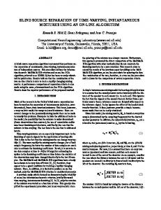
Although from the effect of the noise and small correlations among the source signals, (3) does not hold in practice. We implemented in the way to minimize the off-diagnal components of the matirices BRxx (τi )B T . In order to obtain B, we use the algorithm which only needs straightforward calculations[6]. It consists of two procedures, sphering and rotation. (Fig.1)
Sphering
Rotation
x’’2
x2’
x2 τn
x1
τ1 τ0
τn
x1’
τ1 τ0
τn
x’’1
τ1 τ0
Figure 1: Sphering and Rotation Sphering is a procedure to obtain a matrix V which satisfies, V Rxx (0)V T = I
(4)
and rotation is a procedure to remove off-diagonal elements of correlation matrices with an orthogonal transformation. The implementation is to find an orthogonal matrix C which minimizes r � � � � �(CV Rxx (τl )V T C T )ik �2 ,
(5)
l=1 i�=k
where (∗)ik is the ik-element of a matrix. Cardoso and Souloumiac gave an implementation [1] with Jacobi-like algorithm to obtain C. Finally, matrix B is given by B = CV . An advantage of this method is that it uses only the second order statistics and fixed amount of computation.
3
Proposed Method
In this section, the detail of the algorithm is shown along with the flow of it. First, the windowed-Fourier transform is applied to convolutive mixed signals, ˆ x(ω, ts ) =
�
e−jωt x(t)w(t − ts ), (6)
t
ω = 0,
1 N −1 N 2π, . . . , N 2π,
ts = 0, ∆T, 2∆T, . . .
where ω denotes the frequency and N denotes the number of points of the discrete Fourier transform, t s denotes the window position, w is a window function (we used Hamming window) and ∆T is the shifting interval of moving ˆ ˆ ω (ts ) = x(ω, ˆ windows. Let us redefine a x(ω, ts ) for a fixed frequency ω as x ts ). If the window length is long enough compared to the impulse response of A(t), the relationship between observations and sources can be approximated as, ˆ s(ω, ts ), ˆ ω (ts ) = A(ω)ˆ x
(7)
ˆ where A(ω) is the Fourier transform of operator A(t), and sˆ(ω, ts ) is the windowed-Fourier transform of s(t). This shows that for fixed ω, a convolutive mixture is simply an instantaneous mixture. We extend the algorithm in §2 to complex values by substituting a Hermite matrix for a symmetric matrix, and apply it for each frequency. As the result, we have a separated time sequence, ˆ ω (ts ) = B(ω)x ˆ ω (ts ). u
(8)
Since BSS algorithms cannot solve the ambiguity of amplitude and permuˆ ω (ts ) along with ω, amplitudes are tation, even if we put each component of u irregular and different independent sources will be mixed up. The problem of irregular amplitude can be solved by putting back the separated independent components to the sensor input with the inverse matrices B(ω)−1 . Let us define vˆω (ts ; i) as, vˆω (ts ; i) = B(ω)−1 (0 . . . 0, u ˆi,ω (ts ), 0 . . . 0)T ,
i = 1, . . . , n
(9)
ˆ ω (ts ) where vˆk,ω (ts ; i) represents the input of i-th independent component of u into the k-th (k = 1, . . . , n) sensor. We applied B(ω) and B(ω)−1 to obtain vˆω (ts ; i), therefore vˆω (ts ; i) has no ambiguity of amplitude. Remaining problem is permutation. We made an assumption that even for different frequencies, if the original souce is the same, the envelopes are similar. We utilize this idea for solving the permutation. Let us define an operator E to take the envelope as, E vˆω (ts ; i) =
1 2M
ts� +M
n �
t�s =ts −M
k=1
|ˆ vk,ω (t�s ; i)|,
(10)
where M is a positive constant and vˆk,ω (ts ; i) denotes the k-th element of vˆω (ts ; i). Inner product and norm are defined as � E vˆω (i) · E vˆω� (k) = E vˆω (ts ; i)E vˆω� (ts ; k), (11) ts
� Evω (i) = E vˆω (i) · E vˆω (i),
(12)
and we define the similarity between two envelopes as the following, sim(ω) =
� E vˆω (i) · E vˆω (k) . E vˆω (i) E vˆω (k)
(13)
i�=k
Using these operations, we solve the permutation as follows: Solve the Permutation
! = sort(ω, sim)
sorting ω to be sim(ω1 ) < · · · < sim(ωN )
for i = 1 to n do
yˆω
1
ˆω1 (ts ; i) (ts ; i) := v
done for l = 2 to N do for i = 1 to n do
n
ˆωk (i� ) · σ(i) := argmaxi� E v yˆωl (ts ; i) := vˆωl (ts; σ(i))
�P
l−1 k=1
�o
E yˆωk (i)
done done
As a result, we obtain separated spectrograms as yˆω (ts ; i). Applying inverse Fourier transform, finally we get a set of separated sources y(t; i) =
1 � � jω(t−ts ) 1 · e yˆω (ts ; i), 2π W (t) t ω
i = 1, . . . , n
(14)
s
� where W (t) = ts w(t − ts ). Note that each � yk (t; i) represents a separated independent component i on sensor k, and i y(t; i) = x(t) holds.
4 4.1
Experimental Results Artificial Data
We show a result of an experiment on a set of data which were recorded separately and mixed on a computer. Since we wanted to simulate the general problem of recording sounds in a real environment, we built a virtual room as Fig.2 and calculated reflections and delays. We supposed that each wall, floor and ceil reflect the sound once and the strength of sounds varies in proportion to the inverse square of the distance. The strength of the reflection is 0.1 in power for any frequency.
3
Source 2 2 3
Source 1
2
1.4 1.7
3
Mic. 1 1.5
7
Mic. 2 0.4 2
4.5
7
Figure 2: Virtual Room Since we know the true sources and the mixing rates, we evaluate the performance with SNR (Signal to Noise Ratio) which is defined as, signali (t; k) = aik sk (t), errori (t; k) = yi (t; k) − signali (t; k) � signali (t; k)2 . SNRik = 10 log10 �t 2 t errori (t; k) We applied our algorithm, changing the window length from 8msec to 32msec. 1
y1(t;1)
0 −1
1
x (t) 1
y2(t;1)
0 −1
0
0.1
0.2
0.3
0.4
0.5 Time(sec)
0.6
0.7
0.8
0.9
0.2
0.3
0.4
0.5 Time(sec)
0.6
0.7
0.8
0.9
1
0
0.1
0.2
0.3
0.4
0.5 Time(sec)
0.6
0.7
0.8
0.9
1
0
0.1
0.2
0.3
0.4
0.5 Time(sec)
0.6
0.7
0.8
0.9
1
0
0.1
0.2
0.3
0.4
0.5 Time(sec)
0.6
0.7
0.8
0.9
1
1
y1(t;2)
0 −1
0.1
0 −1
1
1
x2(t)
0
1
0
0.1
0.2
0.3
0.4
0.5 Time(sec)
0.6
0.7
0.8
0.9
0 −1
1
1
y2(t;2)
0 −1
a
b Figure 3: a: Mixed Signals in a Virtual Room b: Separated Signals The SNRs of these results are shown in Tab. 1. Our approach with the window length of 32msec gave the best SNRs. Mixed inputs (Fig.3.a) and separated signals (Fig.3.b) are shown. Signals were clearly separated. Table 1: SNRs (dB) for Separated Signals (∆T is 1.25msec and r in (3)is 40) SNR11 SNR12 SNR21 SNR22 8msec 4.36 6.32 11.94 11.66 Window length 16msec 4.72 6.65 12.66 12.52 32msec 6.47 7.30 14.40 13.19
4.2
Real-room Recorded Data
Finally, we applied the algorithm to the data recorded in a real environment. The data was provided by Prof. Kota Takahashi in the University of ElectroCommunications. Two males were repeating different phrases simultaneously in a room and their voices were recorded with two microphones with 44.1kHz for 5sec then down-sampled to 16kHz. Inputs are shown in Fig.4.a.
We applied our algorithm to this data. Window length was 32msec (512 points), ∆T was 1.25msec and r was 40. The result is shown in Fig.4.b. We show the separated signals in the graphs. We heard them and they were separated clearly. 1
y (t;1) 1
0 −1
1
x1(t)
y2(t;1)
0 −1
0
0.5
1
1.5
2
2.5 Time(sec)
3
3.5
4
2
1
1.5
2
2.5 Time(sec)
3
3.5
4
4.5
0
0.5
1
1.5
2
2.5 Time(sec)
3
3.5
4
4.5
0
0.5
1
1.5
2
2.5 Time(sec)
3
3.5
4
4.5
0
0.5
1
1.5
2
2.5 Time(sec)
3
3.5
4
4.5
1
y (t;2)
0 −1
0.5
0 −1
4.5
1
x (t)
0
1
1
0
0.5
1
1.5
2
2.5 Time(sec)
3
3.5
4
0 −1
4.5
1
y2(t;2)
0 −1
a
b
Figure 4: a: Recorded Signals in a Real Room b: Separated Signals
5
Conclusion
We proposed a BSS algorithm for speech signals. Our algorithm only uses straightforward calculation, and it includes only a few parameters to be tuned. Through the experiments, the algorithm worked very well for the data mixed on the computer and also for the real-room-recorded data. We haven’t shown other results but they are available at http://www.islab.brain.riken.go.jp/~shiro/blindsep.html This algorithm is easy for hardware implementation, and we are now working for it. We are also working for realizing its on-line version. An on-line algorithm will make it possible to track walking speakers. In this article, we used the envelope of the signals to construct independent spectrograms form spectrograms form separated frequency components. It may be possible to use the continuity of de-mixing matrices between close frequency channels.
References [1] J.-F. Cardoso and A. Souloumiac. Jacobi angles for simultaneous diagonalization. SIAM J. Mat. Anal. Appl., 17(1):161–164, 1996. [2] S. C. Douglas and A. Cichocki. Neural networks for blind decorrelation of signals. IEEE Trans. Signal Processing, 45(11):2829–2842, 1997. [3] T.-W. Lee, A. Ziehe, R. Orglmeister, and T. Sejnowski. Combining time-delayed decorrelation and ICA: towards solving the cocktail party problem. In Proceedings of ICASSP’98, 1998. [4] L. Molgedey and H. G. Schuster. Separation of a mixture of independent signals using time delayed correlations. Phys. Rev. Lett., 72(23):3634–3637, 1994. [5] P. Smaragdis. Blind separation of convolved mixtures in the frequency domain. In International Workshop on Independence & Artificial Neural Networks, University of La Laguna, Tenerife, Spain, 1998. [6] A. Ziehe. Statistische verfahren zur signalquellentrennung. Master’s thesis, Humboldt Universit¨ at, Berlin, 1998. (in German).