Loss function for blind source separation ... - Semantic Scholar

Loss Function for Blind Source Separation-Minimum Entropy Criterion and Its Generalized Anti-Hebbian Rules Hsiao-Chun Wu

Jose C. Principe

NEB 486, New Engineering Building Computational NeuroEngineering Laboratory Department of Electrical and Computer Engineering University of Florida, FL 3261 1

NEB 45 1, New Engineering Building Computational NeuroEngineering Laboratory Department of Electrical and Computer Engineering University of Florida, FL 326 11

wu @ cnel.ufl.edu, or richardw0srl.css.mot.com

principe @cnel.ufl.edu

John G. Harris

Jui-Kuo Juan

NEB 453, New Engineering Building Computational NeuroEngineering Laboratory Department of Electrical and Computer Engineering University of Florida, FL 3261 1

Motorola Labs Florida Communications Research Lab Room 2141 8000 W Sunrise Blvd, Plantation, FL 33322 ejj0040email.mot.com

harris@ cnel.ufl.edu

Abstract Blind source separation has been intriguing many scientists. In adaptive signal processing, LMS (kast-mean squared) algorithm has long been used in signal enhancement and noise cancellation but it cannot ovexome the d$jiculty caused by the signal leakage into the reference input. Hence we have to explore more general statistical properties about the observed signals. This view corresponds to a statistical modeling of the signals using statistical measures such as a lossfunction, which is differentfrom the mutual information. This paper will propose a new loss function based on generalized Gaussian distributionfamily and derive nav simple adaptive learning rules. Our separator based on the new generalized “anti-Hebbianrules” is alsojustified by the simulation on both artificial and real data with good pelfonnance.

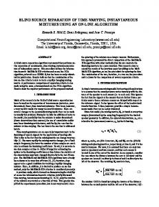
Figure 1. Mixing and separating. Unobserved sources: s, observations: x, estimated source signals: y.

The observations are obtained at the output of several sensors, which receive different linear convolutive combinations of the source signals. Blind source separation (BSS) denotes the following practical problem: by observing the mixtures of sources assumed independent,we try to recover the sources [13. In the real situation, neither a priori information of the transfer function from the sources to sensors is available, nor are the source signals observable. However, based on the statistical independence assumption, we can often achieve plausible approaches to separate the sources from the mixture.

1. Introduction Blind signal separation (BSS) is recovering unobserved signals or ‘sources’ s(t)from several observed mixtures x(t) as depicted in Figure 1.

The most straightforward independence measure is the mutual information. The mutual information is described as the difference between the sum of marginal entropies H(yi)

0-7803-5529-6/99/$10.00 01999 IEEE

910

and joint entropy HO1,y2, ....,YN).The mutual information among N random variables yl, y2, ...,yNis defined by

to obtain

N

I(y1, y29

...I

YN)

=

H ( y i ) - H ( y ] , Y2t

YN)1

(l)

i= 1

where H(ri) and H b l , y2, ...,y~)are marginal and joint entropy, respectively. The mutual information is always greater than or equal to zero. It is zero when all the random variables yl, y2, ..., yN are statistically independent. When the sources are mixed in form of a convolutive model, the mutual information of Equation (1) is not a good criterion for learning systems since it is difficult to estimate the joint entropy HOl, y2, ....,yN). There has been no general non-Gaussian joint probability density model available so far. Hence we need to look for other contrast functions for blind source separation. Recently, an alternative information measure has been proposed for blind source separation and deconvolution [2-4] and it has been empirically justified for source separation. This contrast function is associated with the marginal entropy of the output and the constraintof the weight matrix. Using this new contrast function as our information measure for the blind source separation, we apply the generalized Gaussian distribution model and derive the Generalized Anti-Hebbian Learning (GAL) rules.

2. Distribution Model In this section, we will discuss a family of distribution models for our use, namely, generalized Gaussian distributions.The generalized Gaussian model was named by

Miller and Thomas [5] and used in detection theory as a model for non-Gaussian noise. It is a family of symmetric probability distributions defined by

3. Loss Function for Statistical Independence For a convolutive mixture, the observations are denoted by

xi(?) and the sources sxf). Let r(f) and s(?) be the vectors [xl(t), x2(?),

...., xnr(f)lTand[sl(t),s2(f), ..., slv