Multirate sampling has been mainly used to reduce computation effort in ... Model
Predictive Control (MPC) multirate controller in which a multivariable plant is.
IJC '12
Model-Based Control of Networked Distributed Systems with Multirate State Feedback Updates Abstract. This paper presents a model-based multirate control technique for stabilization of uncertain discrete-time systems that transmit information through a limited bandwidth communication network. This model-based multirate approach is applied to two networked architectures. First, we discuss the implementation of a centralized control system with distributed sensing capabilities and, second, we address the problem of stabilization of networks of coupled subsystems with distributed sensors and controllers. In both cases we provide necessary and sufficient conditions for stability of the uncertain system with multirate model updates. Furthermore, we show that, in general, an important reduction of network bandwidth can be obtained using the multirate approach with respect to the single rate implementations. Keywords: multirate systems;; networked control systems;; distributed control;; lifting techniques.
1. Introduction In recent years there has been a strong interest in the analysis, development, and controller synthesis for networks of interconnected systems. Examples of such systems can be found in a wide variety of applications such as: power networks, multiagent robotic systems and coordination of autonomous vehicles, large chemical processes comprised of several subsystems interacting one with each other, and also in areas that consider economic and/or social systems. In addition, the availability of cheap, fast, embedded sensor and controller subsystems that are capable to communicate via a shared digital network allow for the different subsystems to share their local information with other (possibly the rest of) subsystems so it can be used to achieve a common objective in a more efficient way (Camponogara, et.al. 2002;; Dunbar 2007;; Sinopoli, et.al. 2003). The support of the National Science Foundation under Grant No. CNS-1035655 is gratefully acknowledged.
1
However, digital communication networks have limited bandwidth and not all agents can communicate at a given time instant. It becomes necessary to be able to schedule the broadcast of information by the different nodes in such a way that bandwidth constraints are not violated (Lian, Moyne, and Tilbury 2001;; Antsaklis, and Baillieul 2007). Different approaches that reduce the necessary network bandwidth have been investigated such as minimum bit rate stabilization (Elia and Mitter 2001), packetized control (Georgiev and Tilbury 2004), and model- based control (Montestruque and Antsaklis, 2003). Multirate sampling has been mainly used to reduce computation effort in sampled data systems (Yu and Yu 2007). The work in (Yu and Yu 2007) provides experimental results of a Model Predictive Control (MPC) multirate controller in which a multivariable plant is approximated by 3 single-output models which are modeled and sampled at different rates. The main purpose in this work is to sample the output representing the slow dynamics of the system at a lower rate in order to reduce the dimension and complexity of the optimization problem at those sampling instants when only the fast dynamics are sampled. Other references concerning the implementation of multirate MPC algorithms are (Scattolini and Schiavoni 1995) and (Lee, Gelormino, and Morari 1992). The multirate implementation generalizes the dual-rate approach frequently used in sampled- data and networked systems (Li, Shah, and Chen 2002;; Ding and Chen 2004;; Ding and Chen 2005;; Tange 2005) where two different rates are used in the control system. These two rates correspond each one to the actuator (fast rate) and the sensor (slow rate). In the dual-rate approach it is assumed that the entire output vector is measured and sent trough the network at the same time instant.
2
Multirate systems have also been studied using different approaches. The authors of (Sezer and Siljak 1990) provide stabilizability conditions for continuous-time Linear Time Invariant (LTI) systems using decentralized controllers and sampling the system inputs using different sampling rates. Vadigepalli and Doyle (2003) developed a multirate version of the Distributed and Decentralized Estimation and Control (DDEC) algorithm in (Mutambara and Durrant-Whyte 2000) for large scale process based on model distribution and internodal communication. The model distribution provides a definition of the states of interest to be estimated locally by each node using measurements that are sampled periodically using different intervals at each node. Communication between nodes is used in order to share information due to the interactions between local subsystems resulting from the model decomposition overlapping states. The present paper extends initial results described in (Garcia and Antsaklis 2010) to consider two important architectures in control systems that communicate their measurements using a limited bandwidth communication channel. The first problem considers the control of large scale uncertain systems with multiple outputs and spatially distributed sensing implementation. In this type of implementation the sensors that measure different elements of the state vector can be located at distant positions. A limited bandwidth communication network is used to send all sensor measurements to the controller. In order to schedule the sampling and sharing of information and to increase the sampling intervals at each sensor node as much as possible we implement a multirate sampling scheme. The results concerning this problem provide a simple approach to address robustness to parameter uncertainties using multirate sampling in contrast to (Yu and Yu 2007;; Scattolini and Schiavoni 1995;; Lee, Gelormino, and Morari 1992;; Li, Shah, and Chen 2002;; Tange 2005;; Sezer and Siljak 1990;; Vadigepalli and Doyle 2003) where it is assumed that the plant and model parameters are the same.
3
The second problem that is analyzed in the present paper corresponds to a decentralized architecture in which it is necessary to stabilize a set of coupled, uncertain, and unstable dynamical systems. In this architecture a Local Control Unit (LCU) is implemented within each subsystem and it is assumed that each subsystem is able to measure its own state at all times but it is allowed to broadcast its measurements to other subsystems only at certain instants according to its assigned update rate. Similar to the problem described above, we do not restrict the subsystems to use the same update rates but those rates can be all different in general. In order to reduce the necessary network bandwidth for stabilization we follow the Model- Based Networked Control Systems (MB-NCS) approach in Montestruque and Antsaklis (2003;; 2004;; 2005), Lunze and Lehmann (2010), Garcia and Antsaklis (2012), Garcia, Vitaioli, and Antsaklis (2011). In MB-NCS a nominal model of the system is implemented in the controller node to provide estimates of the state of the system for the intervals of time that feedback measurements are not transmitted by the sensor nodes. Similar MB-NCS implementations have been used for distributed systems by Sun and El- Farra (2008;; 2012a;; 2012b), El-Farra and Sun (2009). In (Sun and El-Farra 2008) the authors study the stabilization of coupled continuous-time systems employing the MB-NCS in (Montestruque and Antsaklis 2003) and using a single rate approach which forces all agents to send measurement updates through the network all at the same time instants. That approach was extended in (El-Farra and Sun 2009) and in (Sun and El-Farra 2012a;; 2012b) to the case when a schedule for the updates is pre-assigned but all subsystems still use the same update rate, i.e. a single rate approach in which the agents send updates at different time instants. The approach in our paper offers more flexibility and provides, in general, further reduction of network communication. Each subsystem is allowed to send measurements using its own update rate.
4
Subsystems with slower dynamics or represented by more accurate models are able to use lower update rates and they are not restricted to use the same rates as the subsystems with faster dynamics. The paper is organized as follows. Section 2 provides a background analysis of MB-NCS using single rate. Section 3 considers the centralized control problem using multirate sensor measurements. Section 4 and 5 address the decentralized architecture using single rate and multirate updates, respectively. Section 6 provides an illustrative example for estimating admissible model uncertainties and section 7 concludes the paper.
2. Preliminaries and MB-NCS with single-rate updates We recall a simple result concerning discrete-time LTI systems: Theorem 1 (Antsaklis and Michel 1997). The equilibrium x=0 of system x(k+1)=Fx(k) is asymptotically stable if and only if all eigenvalues of F are within the unit circle of the complex plane, i.e. if O1...On denote the eigenvalues of F, then O j � 1, j 1,..., n .Ŷ Let us consider a discrete-time system and model given, respectively, by:
x(k � 1)
Ax(k ) � Bu (k ) (1)
xˆ (k � 1)
ˆ ˆ (k ) � Bu ˆ ˆ (k ) Ax (2)
with A, Aˆ \ nun and B, Bˆ \ num . The control input is given by u (k )
Kxˆ (k ) . In MB-NCS
measurements of the system which are used to update the model of the system at the controller node. The entire state of the system is sampled periodically. The sampling term refers to the time event in which the sensor measures the state and sends this measurement through the network in order to update the corresponding state of the model. The sampling period used by the sensor is greater or equal than the original operating period of the discrete-time plant. By using this 5
approach we try to reduce the number of samples that are transmitted from the sensor to the model/controller. We search for larger sampling periods, which are integer multiples of the operating period of the system, i.e. if the original period of the system is denoted by T time units then the sampling periods are allowed take values T, 2T, 3T, … In this paper we refer to the sampling periods that the sensors use to measure and update the model as update periods in order to differentiate them from the underlying period of the plant T. The associated rates to the update periods are called therefore update rates. Assume without loss of generality that the underlying period of the plant is T=1. The MB-NCS was studied in (Garcia and Antsaklis 2010) using a lifting technique. The lifting process has the purpose of extending the input and output spaces properly in order to obtain a Linear Time Invariant (LTI) system description for sampled-data, multirate, or linear time-varying periodic systems. Since the lifted system is a LTI system, the available tools and results for LTI systems are applicable to the lifted system as well. For details on the discrete-time lifting technique used in this work refer to Chen and Francis (1995) and to Bittanti and Colaneri (2000) and Kahane, Mirkin, and Palmor (1999) for alternative approaches. A MB-NCS with periodic updates is clearly a linear time-varying periodic system by considering an output x that is equal to xˆ when measurements are not transmitted and equal to x when we have an update. Denote the input and output for the lifted system by u and x respectively and they are given by the following
u (kh)
ªu (kh) º «u (kh � 1) » « » «: » « » ¬u ((kh � h � 1) ¼
6
ª Kx(kh) º « Kxˆ (kh � 1) » « » (3) «: » « » ¬ Kxˆ ((kh � h � 1) ¼
x (kh)
ªI º ª0 «ˆ » «ˆ «A » «B « Aˆ 2 » x(kh) � « AB ˆˆ « » « «: » «: « h �1 » « h�2 «¬ Aˆ »¼ «¬ Aˆ Bˆ
0 ... 0 ... Bˆ ... Aˆ h �3 Bˆ ...
0 º » 0» 0 »» u (kh). (4) : » » 0 »¼
The dimension of the state is preserved and the state equation expressed in terms of the lifted input is given by: Ah x(kh) � ª¬ Ah �1 B
x((k � 1)h)
Ah � 2 B ... B º¼ u (kh). (5)
Theorem 2. The lifted system is asymptotically stable if and only if the eigenvalues of h �1
ˆ ) j (6) Ah � ¦ Ah �1� j BK ( Aˆ � BK j 0
are within the unit circle of the complex plane. Proof. To prove this theorem we note that (5) is the same as the state equation that characterizes the autonomous linear time invariant system: x((k � 1)h)
h �1
ˆ ) j ) x(kh). (7) ( Ah � ¦ Ah �1� j BK ( Aˆ � BK j 0
Equation (7) can be obtained by directly substituting (3) in (5), and then substituting the value of each individual output by its equivalent in terms of the state x(kh), i.e. ˆ (kh) � Bu ˆ (kh) ( Aˆ � BK ˆ ) x(kh) Ax ˆ ) 2 x(kh) xˆ (kh � 2) ( Aˆ � BK (8) xˆ (kh � 1)
:
The resulting equation can be simply expressed as (7). The lifted system is an LTI system and by Theorem 1 it is asymptotically stable if and only if the eigenvalues of (6) have magnitude less than one�Ŷ
7
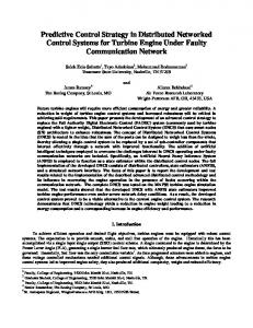
3. Spatially distributed systems with multirate sensor measurements In this section we use the MB-NCS approach and the lifting procedure to establish stability conditions for discrete-time spatially distributed systems when their states are sampled periodically but using different sampling rates. This multirate approach is necessary especially when different sensors are used to measure different elements of the system output, see Figure 1. When the sensors use the same network to transmit their measurements to the controller node then the multirate approach brings important benefits to the operation of the overall networked system. By allowing the sensors to transmit their measurements using different sampling periods we avoid packet collisions and networked induced delays compared to the case when all of the sensors need to sample and transmit at the same instants. Additionally, we will show that in many cases a further reduction in network communication can be obtained by using different update rates for each sensor compared to the single rate case shown in Garcia and Antsaklis (2010). Although the multirate sampling case requires a more complex analysis, the same lifting approach can be used in order to find a system representation for the LTI equivalent (lifted) system.
8
Figure 1. Networked control system with centralized controller and distributed multirate sensor measurements. Consider a multi-output system depicted in Figure 1. In this case we do not assume that a single sensor measures all states at the same time;; instead we consider a spatially distributed system for which different sensors measure different elements of the state and send this information to the centralized controller at different rates. The state of the model is partially updated according to the information that is received at any given update instant. In what follows we will provide details on how the state of the model is partially updated and how to obtain the response of the corresponding lifted system. The lifted system state equation directly provides necessary and sufficient conditions for the stability of the multirate system. We consider an N-partition of the state of the system (1), and the model (2) likewise, according to the number of sensors that are used to obtain measurements:
9
x
where xi , xˆi \ ni ,
N
¦ ni
ª x1 º «x » « 2 » , xˆ «# » « » ¬ xN ¼
ª xˆ1 º « xˆ » « 2 » (9) «# » « » ¬ xˆ N ¼
n . In general, each subset of the system state may have different
i 1
dimensions. Let si represent the update period that sensor i uses to send measurements in order to update the corresponding part of the model state xˆi . Let s represent the minimum common multiple of all si . In order to obtain the response of the multirate system using the model-based control input with partial updates we define all the update instants within a period s by arranging the periods
si and its multiples up to before s in increasing order as follows: s1 , 2 s1 ,..., (r1 � 1) s1 s2 , 2 s2 ,..., (r2 � 1) s2
(10)
# sN , 2 sN ,..., (rN � 1) sN where ri
s si
for i=1…N represents the relative update rate compared to the update rate given by
the period s. Let hi for i=1…p-1 represent the update instants in increasing order, where p is the total number of update instants within a period s including the update at time s. Note that at any given instant one or more sets of states xˆi can be updated. This procedure can be better shown trough a simple example.
10
Consider the state of a system that is partitioned into three subsets x1 , x2 , x3 with corresponding periods s1
3, s2
4, s3
6 . Then we proceed to define all update instants within
a period s=12, as follows:
h1
3 s1
h2
4
h3
6 2 s1
h4
8 2 s2
h5
9 3s1
s2 s3 (11)
Note that at the time instant h3 we have two partial updates for this example. Let us define, in general, the partial update matrices:
Ii
ª0 0 «0 I ni « «¬0 0
0º (12) 0 »» 0 »¼
that is, the ith partial update matrix I i \ nun contains an identity matrix at the position corresponding to xi and zeros elsewhere. Define I hi
I i � I j � I k ...
(13)
The matrices I hi represent all updates that happen at time instant hi . Theorem 3. The uncertain system with distributed sensors as shown in Figure 1 with model- based control input and with partial multirate model updates is asymptotically stable for given update periods si if and only if the eigenvalues of p
As � ¦ A i 1
h p � hi
; hi � hi�1U hi �1
are within the unit circle of the complex plane, where
11
(14)
hi � hi �1 �1
¦
; hi � hi�1
0, U h0
j 0
ˆ ) ( I � I hi )( Aˆ � BK
U hi
with h0
ˆ )j Ahi � hi�1 �1� j BK ( Aˆ � BK
I , hp
hi � hi �1
i
U hi �1 � I hi ( A � ¦ A hi
(15) hi � hq
q 1
; hq � hq�1U hq �1 )
s .
Proof. Let us consider the beginning of a period s. At this time instant all sensors send measurements and we have that xˆ (ks )
x(ks ) . At the time of the first update after time ks, that
is, at time ks � h1 we have: h1 �1
ˆ ) j ) x(k ) ( Ah1 � ; ) x(ks ) x(ks � h1 ) ( Ah1 � ¦ Ah1 �1� j BK ( Aˆ � BK h1 j 0
(16)
and the model state after the update has taken place is given by: ˆ ) h1 � I ( Ah1 � ; )) x(k ) U x(ks ). xˆ (ks � h1 ) (( I � I h1 )( Aˆ � BK h1 h1 h1
(17)
Following a similar analysis we can obtain the response of both the system and the model at time
ks � h2 as a function of x(ks � h1 ) and xˆ (ks � h1 ) : x(ks � h2 )
Ah2 � h1 x(ks � h1 ) �
h2 � h1 �1
¦
ˆ ) j xˆ (ks � h ) Ah2 � h1 �1� j BK ( Aˆ � BK 1
j 0
ˆ ) h2 � h1 xˆ (ks � h ) � I x(ks � h ) xˆ (ks � h2 ) ( I � I h2 )( Aˆ � BK h2 1 2
(18)
(19)
but, since both x(ks � h1 ) and xˆ (ks � h1 ) can be expressed in terms of x(ks), we obtain the following: x(ks � h2 ) ( Ah2 � Ah2 � h1 ; h1 � ; h2 � h1U h1 ) x(ks )
(20)
ˆ )h2 � h1 U � I ( Ah2 � Ah2 � h1 ; � ; U )) x(ks ) U x(ks ). xˆ (ks � h2 ) (( I � I h2 )( Aˆ � BK h1 h2 h1 h2 � h1 h1 h2
By following the same analysis for each update instant hi up to hp
12
s we obtain
(21)
p
x((k � 1) s ) ( As � ¦ A i 1
h p � hi
; hi � hi�1U hi �1 ) x(ks ). (22)
Since (22) represents an LTI system then the networked system is asymptotically stable when the eigenvalues of (14 �OLH�LQVLGH�WKH�XQLW�FLUFOH��Ŷ Example 1. Consider the 5th order unstable system given by:
ª �1.05 « 0.35 « A « 0.03 « « 0.06 «¬ 0.035
0.35 0.02 0.35 0.24 º 1.1 0.1 0.035 0.035»» 0.32 0.21 �0.4 0.6 » , B » 0.03 0.3 �0.7 0.55 » 0.03 0.6 0.3 0.2 »¼
ª1 «1 « «1 « «1 «¬1
1º 2 »» 1 » » 2» 1 »¼
ª1 «1 « «1 « «1 «¬1
1º 2 »» 1 » » 2» 1 »¼
Its nominal model is given by:
0.35 ª �1 « 0.35 1 « Aˆ « 0.03 0.35 « « 0.06 0.035 «¬0.035 0.035
0.24 º 0.05 0.035 0.035»» 0.15 �0.45 0.6 » , Bˆ » 0.34 �0.75 0.6 » 0.5 0.3 0.4 »¼ 0.02
0.35
If it were possible to implement a single sensor and send periodic updates, that is, to send the whole state at the same time instants we would need to use a period h