Acceleration of Reinforcement Learning by Using State ... - CiteSeerX

Acceleration of Reinforcement Learning by Using State Transition Probability Model Kei Senda, Shinji Fujii, Syusuke Mano Graduate School of Natural Science and Technology, Kanazawa University 2-40-20 Kodatsuno, Kanazawa, Ishikawa 920-8667, Japan

Abstract. The Q-learning is one of typical reinforcement learning methods. Since the Q-learning requires huge amounts of time to solve a problem, this study proposes acceleration methods. This study introduces two approaches based on the value iteration method of the dynamic programming to accelerate the learning. One is the use of proper estimation of the state transition probability model and the other is the application of iterative solving methods for an inverse matrix, e.g. , Jacobi’s method, Gauss-Seidel’s method, SOR method, etc. Those allow us to determine the optimal learning factor and to make the learning more efficient than the Q-learning. Numerical simulations show that the proposed methods are effective. Keywords: Q-learning，State transition probability model, Value iteration，Jacobi’s method, Gauss-Seidel’s method，SOR method

1

Introduction

The Q-learning, one of typical reinforcement learning methods, does not need a model of the plant. The Qlearning estimates the Q-factor of a state-action pair, which evaluates the action at the state. Action is then selected according to the estimated Q-factor. In the Q-learning, the learning means obtaining the Q-factors that provide the optimal actions. Starting with the unknown Q-factors, The Q-factors are updated through trialand-error procedure. Finally, the convergence of the Q-factors to the true values is guaranteed (Bertsekas et al. 1996, Sutton et al. 1998). However, how to set parameters, e.g. , the learning rate, has not been established. Hence, it often takes a very long time to learn. In addition to that, to realize feasible learning, many problems are left in the learning algorithm. The Q-learning is associated with the dynamic programming (DP) and derived from value iteration that is one of DP methods (Bertsekas et al. 1996). The value iteration is a model-based method, whereas the Q-learning realizes a model-free method by an approximation of the model. But, the Q-learning converge much slower than value iteration because of the approximation. We propose a more effective learning algorithm considering value iteration with model estimation. This study sequentially estimates the model by the Robbins-Monro stochastic approximation method (Kushner et al. 2003), whereas there are some model estimation methods (Ishii et al. 2002, Brafman et al. 2002). As a result, the parameter of learning rate is properly determined. Furthermore, we show that estimating of the Q-factors by the value iteration can be transformed into solving a large size of simultaneous linear algebraic equations. The corresponding DP iteration is regarded as an iterative solving method. This study tries to accelerate the learning speed by applying effective iterative solving methods, i.e. the Jacobi’s method, the Gauss-Seidel’s method, and the SOR method. The resulting value iteration method using an agent is regarded as one of algorithms called asynchronous value iteration (Bertsekas 1982, Bertsekas et al. 1989, Williams et al. 1990). Its convergence is guaranteed on certain conditions, and its learning speed is accelerated from the Q-learning. In this paper, the treated reinforcement learning problem is firstly defined. The structure of the Q-learning is explained. Considering the structure, An algorithm using the value iteration with proper model estimation is proposed, which is more effective than the Q-learning. Furthermore, the more effective value iteration is made by applying the iterative solving methods of a inverse matrix. As a result, the learning speed is accelerated. The obtained algorithm is applied to an 11×11 maze problem. Numerical simulations show that the proposed methods are effective.

2

Reinforcement Learning Problem

Following a general DP formulation (Bertsekas et al. 1996), we have a discrete-time dynamic system. State si and action uk are discrete variables that are elements of the finite sets. There are N states, denoted by s1 , s2 , . . . , sN , plus possibly an additional termination state, denoted by s0 . There are K actions, denoted by u1 , u2 , . . . , uK . At state si , the choice of an action uk specifies the state transition probability pij (uk ) to

the next state sj , and we incur a cost g(si , uk , sj ). The systems discussed here are not obviously dependent on time. When pij (uk ) of transition to sj is dependent on only current si and uk , the system satisfies the Markov property and is called a Markov decision process (MDP). The action depends on the state, and a function mapping the state into the action is called a policy. In infinite horizon problems defined later, most interesting policies are time-independent stationary policies. Hence, stationary policies are considered in this study. The probability to select a action based on the policy µ is denoted by π(si , uk ), called the action selection probability. We can distinguish between finite horizon problems, where the cost accumulates over a finite number of stages M , and infinite horizon problems, where the cost accumulates indefinitely. The problems in this study are considered as infinite horizon problems to be solved by learning. In infinite horizon problems, a cost accumulates additively over time. At the m-th transition, we incur a cost αm g(si , uk , sj ), where α is a scalar with 0 < α ≤ 1, called the discount factor. The total expected cost (Q-factors) starting from an initial state si and an initial action uk , and using a policy µ is ¯ " M −1 # X ¢¯ ¡ m µ 0 m m m+1 ¯ 0 Q (si , uk ) = lim E α g s , µ(s ), s ¯ s = si , µ(s ) = uk . M →∞ ¯ m=0

PK The problems is often formulated with J(si ) = k=1 π(si , uk )Q(si , uk ) called J-factors. But, in this study, the Q-factor is consistently used. The optimal Q-factor is denoted by Q∗ (si , uk ) = minµ Qµ (si , uk ). We say that µ is optimal if Qµ (si , uk ) = Q∗ (si , uk ) for all states si and actions uk . The optimal Q-factor satisfies the ½ ¾ following form. N X ∗ ∗ Q (si , uk ) = pij (uk ) g(si , uk , sj ) + α min Q (sj , uk0 ) (1) uk 0

j=0

We define a vector of elements Q(si , uk ) as Q (see appendix). The vector of the Q-factors with policy µ is denoted by Qµ . In this study, the discussed problems can be considered as stochastic shortest path problems that are a class of the infinite horizon problems. In the problems below, we assure that α = 1 but there is an additional state s0 (goal), which is a cost-free termination state, i.e. p00 (uk ) = 1, g(s0 , uk , s0 ) = 0 for all actions uk . We are interested in problems where reaching the termination state is inevitable, at least under an optimal policy. Thus, the essence of the problem is how to find the optimal policy minimizing Qµ (si , uk ) under those conditions.

3

Acceleration of Learning by Using State Transition Probability Model

3.1

Value Iteration

A mapping H that transforms the vector Q into a scalar is defined to find the solution of Eq. (1): ½ ¾ N X 0 (HQ) (si , uk , `ik + 1) ≡ pij (uk ) g(si , uk , uj ) + min Q(sj , uk , `ik ) , uk 0

j=0

(2)

where `ik is the update count of Q(si , uk ), which is denoted only in case of necessity. The H is viewed as a mapping that transforms all elements of the vector Q into themselves. The composition of the mapping H with itself m times is denote by H m : ¡ ¢ H m Q = H H m−1 Q The mapping H is applied ∞ times, where Q(s0 , uk ) = 0 for all actions uk : Q∗ = lim H m Q

(3)

m→∞

Under proper assumptions, Q∗ calculated by the above equation satisfies Eq. (1) for the stochastic shortest path problem (Bertsekas 1995, Bertsekas et al. 1996). The DP iteration that calculates Q∗ starting from some Q is called value iteration. Even if pij (uk ) or observations include errors, the following form is sometimes used to bring the value iteration close to an exact solution, which is the more general form of Eq. (2): ½ ¾ N X Q(si , uk , `ik + 1) = (1 − γ)Q(si , uk , `ik ) + γ pij (uk ) g(si , uk , sj ) + min Q(sj , uk0 , `jk0 ) , (4) j=0

where γ (γ ∈ (0, 1]) is learning rate.

uk0

3.2

Policy Iteration

In this algorithm, we generate a sequence of new policies µ1 , µ2 , . . ., starting from a policy µ0 . To find the solution Qµm of the simultaneous linear algebraic equations for the given policy µm ( ) N K X X µm µm Q (si , uk ) = pij (uk ) g(si , uk , sj ) + π(si , uk0 )Q (sj , uk0 ) , (5) k0 =1

j=0

the following mapping Hµm is used as same as the value iteration. ( ) N K X X (Hµm Q) (si , uk , `ik + 1) ≡ pij (uk ) g(si , uk , sj ) + π(si , uk0 )Q(sj , uk0 , `ik )

(6)

k0 =1

j=0

The Qµm is obtained when the mapping H µm is applied ∞ times, where Q(s0 , uk ) = 0 for all actions uk . Qµm = lim H m µm Q

(7)

m→∞

This procedure is called a policy evaluation step (PES). To compute a new policy µm+1 , µm+1 (si ) = arg min Qµm (si , uk ), uk

∀ i,

(8)

is performed. This is called a policy improvement step (PIS). The step is repeated with µm+1 in place of µm unless we have the policy µm satisfying Qµm+1 = Qµm . This algorithm is called policy iteration. In a practical policy evaluation step, H µm cannot be infinitely applied as Eq. (7). Therefore, the composition is terminated with finite times. The value iteration is the policy iteration whose PES is terminated once Hµm is applied. Hence, the value iteration can be viewed as a special case of policy iteration. The policy iteration depends on how many iterations is executed in the policy evaluation step, and when the policy is updated in the policy improvement step. Therefore, there are various policy iterations.

3.3

Q-learning

The Q-learning algorithm (Sutton et al. 1998) is a typical method of reinforcement learning. It estimates the optimal Q-factors Q∗ (si , uk ) through interactions with the environment by trial and error. When an action uk is taken, a new state sj and cost g(si , uk , sj ) is observed, then the Q-factors is updated as ½ ¾ Q(si , uk ) ← (1 − γ)Q(si , uk ) + γ g(si , uk , sj ) + min Q(sj , uk0 ) , (9) uk 0

where γ ∈ (0, 1]. Suppose that the system is modeled as a finite MDP, and all actions are selected enough times. Then, it is guaranteed that the estimations Q converge to the optimal values with probability 1, and that the optimal actions are obtained. This study uses the ²-greedy policy (Sutton et al. 1998), to select the action during the learning. Under the ²-greedy policy, an action is selected randomly with probability ², the optimal action is chosen with probability (1 − ²) by using the current estimation of the Q-factors. The updating rule Eq. (9) of the Q-learning is an approximation formula of Eq. (4). In Eq. (9), pij (uk ) is replaced with a state transition caused by the last action (Bertsekas et al. 1996). The Q-learning is the approximate calculation and how to select γ and ² has not been established. Hence, it generally spends much time for the learning to converge.

3.4

Accelerated Learning Method Using State Transition Probability Model

Consider that the state transition probability is unknown in the value iteration as well as the Q-learning. The estimation pij (uk , zik ) of the state transition probability is used. When the agent observes a state transition (si , uk , sj ), the state transition probability is estimated as pi (uk , zik + 1) = (1 − β)pi (uk , zik ) + βI j ,

β≡

1 , zik + 1

(10)

where β is a step size parameter, zik is the count to select state-action pairs (si , uk ), I j is a vector with N elements whose j-th element is 1 and the others are zeros. The larger zik is, the more accurate the state transition probability becomes. The definition of the matrix pi is shown in the appendix. The β is arbitrary in the former equation of Eq. (10), whereas this studyPdetermines the optimal β based on the Robbins-Monro stochastic N approximation algorithm. The condition j=0 pij (uk ) = 1 is automatically satisfied in this updating rule. The estimation of pij (uk ) by Eq. (10) is used in the iteration of Eq. (2). By rearranging the obtained iteration, the following updating rule is derived:

½ ¾ ´ ˆ Q(si , uk ) = (1 − β) HQ (si , uk , zik ) + β g(si , uk , sj ) + min Q(sj , uk0 )

(11)

½ ¾ N ´ X ˆ pij (uk , zik ) g(si , uk , sj ) + min Q(sj , uk0 , `ik ) HQ (si , uk , `ik + 1, zik ) ≡

(12)

³

uk 0

³

uk 0

j=0

The parameter β in the learning rule is properly determined by the Robbins-Monro stochastic approximation algorithm that is often used to estimate the state transition probability, i.e. the model of controlled plant. We ˆ have HQ = Q at the learning convergence, and the Q-factors converge to the true values. Then, Eq. (11) becomes the same as Eq. (9) that is the updating rule of Q-learning. The estimation of Eq. (10) is similarly applied to the state transition probability of Eq. (6). This also gives the updating rule based on the policy iteration. The learning rules proposed here are generalization of the value iteration and the policy iteration. This methods based on the Robbins-Monro stochastic approximation algorithm have superior properties, e.g. to determine parameter β that is equivalent to learning rate γ and to satisfy the condition that the summation of state transition probability should be one.

4

Acceleration of Learning by Efficient Policy Evaluation

4.1

Relation between Policy Evaluation and Inverse Matrix Calculation

A matrix description of Eq. (5) is ¯ +P ¯ ΠQµ , Qµ = G

(13)

¯ P ¯ , and Π are matrices composed of the cost g(si , uk , sj ), the state transition probability pij (uk ), where G, and the action selection probability π(si , uk ), respectively (see appendix). Eq. (13) is a large size of linear algebraic equations, and Qµ is provided by ¯ Π)−1 G ¯ ≡ A−1 G, ¯ Qµ = (I − P (14) ¯ and Π vary during the learning process. The above discussion shows that the policy evaluation step where P calculating Qµ by Eq. (7) is viewed as the iterative solving method of Eq. (14). The value iteration and the policy iteration include the policy evaluation step. Hence, we propose learning methods accelerated by applying effective solving methods of algebraic equations. We concretely apply the Jacobi’s method, the Gauss-Seidel’s method, and the SOR method that are typical iterative solving methods (Varga 1962, Young 1971).

4.2

Effective Policy Evaluation Methods

4.2.1 State-Action Pairs and Timing to Update This study is particularly interested in which state-action pair of the Q-factor should be selected and when it should be updated. The way to select a state-action pair can be categorized into 3 classes. The timing to replace Q-factors with new ones can be categorized into 3 classes. The classification is shown in Table 1．As a special case of the cyclic type and the batch type in the table, to update all state-action pairs at the same time is called synchronous type. The other type is called asynchronous type. 4.2.2 Policy Evaluation Method A new base mapping is defined as (F Q) (si , uk , `ik + 1)

( ) N K X X 1 ˆ j , uk0 , `ik )(1 − Iij Ikk0 ) , (15) ≡ pij (uk ) g(si , uk , sj ) + π(sj , uk0 )Q(s 1 − pii (uk )π(si , uk ) j=0 0 k =1

Table 1. Classifications based on selection of state-action pairs and timing of update

Selection of state-action pairs

Timing of update

Cyclic type : determined order Sequential type : after each Q-factors calculation Agent type : experiential order of agent Batch type : after every plural Q-factors calculations Random type : random order Episodic type : after agent goals

where Iij is called identity-indicator function, witch is 1 if i = j but is 0 otherwise. When pij (uk ) is known and π(si , uk ) is fixed, the iteration of Eq. (15) is particularly called Jacobi’s method. The feature of the Jacobi’s method is that the update is synchronous type like the mapping F , where to obtain the left-hand value at the update counts `ik + 1, all quantities in the right-hand should be at the update counts `ik . The asynchronous update can be considered as contrasted with synchronous algorithms like the Jacobi’s method. One of the methods is to use the latest calculated value independent of the update counts. For example, there exists the updating rule ³ ´ ˆ (si , uk ) Q(si , uk ) = F Q (16) ˆ the latest Q-factors independent of the update counts in the right-hand side. When pij (uk ) is by using Q, known and π(si , uk ) is fixed, the iteration of Eq. (16) is particularly called Gauss-Seidel’s (GS) method. There exists the updating rule ³ ´ ˆ (si , uk ), Q(si , uk ) = (1 − ω)Q(si , uk ) + ω F Q ∀ i, k (17) to accelerate the convergence speed, where ω is called an acceleration factor and needs to satisfy 0 < ω < 2. When pij (uk ) is known and π(si , uk ) is fixed, the iteration of Eq. (17) is particularly called SOR method. The mapping F used in the Jacobi’s method can be replaced with the mapping H. The replacement corresponds to the PES in the policy iteration. The mapping H can be adversely replaced with the mapping F in the value iteration. The algorithm is called Jacobi-UP (update of policy). The Jacobi’s method with the sequential update of model is called Jacobi-UM (update of model). The Jacobi’s method with the sequential update of both model and policy is called Jacobi-UMP (update of model and policy). Hereinafter, the methods are similarly combined and summarized in Table 2.

4.3

Comparison of Policy Evaluation Method

The following three points are to make the learning more efficient. The first point is the efficient updating rule. The mapping F partially solves and calculates the problem and is the more efficient than the mapping H. The second point is asynchronous update. The asynchronous learning rule can adjust the update counts, whereas the synchronous type cannot. The third point is the use of acceleration factor that is used in the SOR method. The above discussion is summarized with respect to the convergence speed of learning in Table 3. Table 2. Classification of policy evaluation method

F H Fˆ ˆ H

¯ is known，Π is fixed ¯ is known，Π is sequentially updated P P Jacobi GS SOR Jacobi-UP GS-UP SOR-UP PES GSPES SORPES VI GSVI SORVI ¯ is sequentially identified，Π is fixed P ¯ is sequentially identified，Π is sequentially updated P Jacobi-UM GS-UM SOR-UM Jacobi-UMP GS-UMP SOR-UMP PES-UM GSPES-UM SORPES-UM VI-UM GSVI-UM SORVI-UM Table 3. Comparison of convergence speed

PES Jacobi GSPES GS SOR updated Q-factor / cyclic / cyclic / cyclic / synchronous synchronous timing of update sequential sequential sequential model known known known known known policy fixed fixed fixed fixed fixed speed of convergence slow   ←→   fast Q-learning GSVI-UM GS-UMP SOR-UMP agent / sequential agent / sequential agent / sequential agent / sequential unknown sequential identification sequential identification sequential identification sequential update sequential update sequential update sequential update slow   ←→   fast

5

Numerical Simulation

5.1

Setting of Simulation Examples

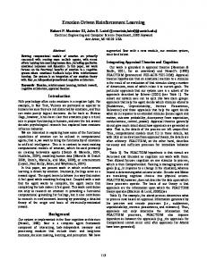
An 11×11 maze shown in Figure 1 is used. Consider that an agent takes four kinds of actions as {up, down, left, right} and the state is its position. All actions result in staying in the same state with probability of 10 %. G

Figure 1. 11 × 11 maze

[Simulation 1]   Suppose that the state transition proba¯ is known and Π is generated by the random policy. bility P The mapping Hµ is compared to Fµ by investigating the convergence speed of the error from the true Q-factor between the PES and the Jacobi’s method. [Simulation 2]   Suppose that the state transition proba¯ is known and Π is generated by the random policy. bility P The convergence speed of the error from the true Q-factor is compared among the PES, the GSPES, the GS method, and the SOR method.

[Simulation 3]   Consider the stochastic shortest path problem for all states to reach the goal (G) with minimum steps. The agent type update is implemented, and the agent moves according to ²-greedy policy of ¯ is unknown at first and is sequentially estimated. Then ² = 0.1. Suppose that the state transition probability P ¯ gradually becomes close to the true value. Suppose that the action selection probability Π is updated with P the greedy policy of the current Q-factors. The convergence speed of the error from the true value are compared ¯ , the J-factor and the Q-factor among the Q-learning, the GSVI-UM，the GS-UMP and the with respect to P SOR-UMP. The speed of obtaining optimal actions is also compared.

5.2

Numerical Results and Considerations

The result of Simulation 1 is shown in Figure 2. This result shows that the mapping Fµ of the Jacobi’s method converges faster than the mapping Hµ of the PES in terms of the error norm from the true Q-factors. The result of Simulation 2 is shown in Figure 3. The acceleration factor ω of the SOR method is 1.6 in this case. This result shows that the SOR method converges the fastest and most effectively among all methods. However, some ω results in Q-factor divergence. The result of Simulation 3 is shown in Figures 4–7. In the figures, each result is an average of 10 times, and ¯ and Π vary, ω is selected to avoid the Q-factor the acceleration factor ω of the SOR method is 1.1. When P divergence by trial and error. Because ω is used about 1 not to destabilize the learning in the point where the Q-factors diverge most easily. However, the Q-factors don’t diverge even if ω is made larger in other points. The learning may be accelerated more if ω can be adequately adapted during the learning. Figures 5 and 7 






ω

Figure 2. Comparison of iterative solving method in the Simulation 1

Figure 3. Comparison of iterative soluving methiod in the Simulation 2

 



 








ω ω





Figure 4. Step history of P error

Figure 5. Step history of J error









ω

ω




Figure 6. Step history of Q error

Figure 7. Step history of Π error

show that the SOR method obtains the optimal actions the fastest for all states. In Figure 6, the convergence speed of the GS method and the SOR method become slow on the way. Because the learning concentrates on the optimal action, and the Q-factors unconcerned with the optimal policy are updated rarely. In other words, the result is because the errors from the all true Q-factors are counted.

6

Conclusions

This paper has mainly studied two approaches to accelerate the learning speed of the Q-learning. One approach has been about the value iteration with the proper model estimation. The model estimation with the appropriate parameter based on the Robbins-Monro stochastic approximation algorithm has made the learning rate properly. The other approach has been applying the iterative solving methods of inverse matrix. The learning has been made more efficient by applying the Jacobi’s method, the Gauss-Seidel’s method, and the SOR method that are typical methods of the iterative solving method. Numerical simulations have shown that the proposed methods, i.e. the GSVI-UM, the GS-UMP and the SOR-UMP can obtain the optimal actions faster than the Q-learning. The SOR-UMP method has had the fastest learning speed of all proposed methods. But, the setting of ω in the SOR method has been difficult, and the method sometimes has resulted in divergence. In the case that the state transition model is estimated, there is a problem that the memory need larger size than the Q-learning. However, we will solve the problem by using a function approximation method.

References Bertsekas, D. P. (1982), “Distributed Dynamic Programming,” IEEE Trans. on the Automatic Control, Vol. AC27, pp. 610–616. Bertsekas, D. P. and Tsitsiklis, J.N. (1989), Parallel and Distributed Computation: Numerical Methods, Prentice-Hall. Bertsekas, D. P. (1995), Nonlinear Programming, Athena Scientific, Belmont, MA. Bertsekas, D. P. and Tsitsiklis, J. N. (1996), Neuro-Dynamic Programming, Athena Scientific. Brafman R. I. and Tennenholtz, M. (2002), “R-max : A General Polynomial Time Algorithm for Near-Optimal Reinforcement Learning,” Journal of Machine Learning Research, Vol. 3, pp. 213–231. Ishii, S., Yoshida, W., and Yoshimoto, J. (2002), “Control of exploitation-exploration meta-parameter in reinforcement learning,” Neural Networks, Vol. 15, No. 4-6, pp. 665–687. Kushner, H. J. and Yin, G. G., Stochastic Approximation and Recursive Algorithms and Applications, SpringerVerlag. Sutton, R. S. and Baro, A. G. (1998), Reinforcement Learning: An Introduction, MIT Press. Varga, R. S. (1962), Matrix Iterative Analysis, Prentice-Hall. Williams, R. J. and Baird, L. C. (1990), “A Mathematical Analysis of Actor-Critic Architectures for Learning Optimal Controls Through Incremental Dynamic Programming,” Proceedings of the Sixth Yale Workshop on Adaptive and Learning Systems, Yale University, pp. 96–101. Young, D. M. (1971), Iterative Solution of Large Linear Systems, Academic Press.

Appendix Definition of Symbol Definitions of symbol for the state transition probability are denoted as pi (uk ) ≡ [ pi1 (uk ), pi2 (uk ), . . . , piN (uk ) ]T , ¯ i ≡ [ pi (u1 ), pi (u2 ), . . . , pi (uK ) ], p ¯ ≡[p ¯1, p ¯2, . . . , p ¯ N ]T . P Definitions of symbol for the action selection probability are denoted as π(si ) ≡ [ π(si , u1 ), π(si , u2 ), . . . , π(si , uK ) ]T , Π(si ) ≡ [ 01 , . . . , 0i−1 , π(si ), 0i+1 , . . . , 0N ]T , Π ≡ [ Π(s1 ), Π(s2 ), . . . , Π(sN ) ], where 0i has K elements, and is the i-th zero vector. Definitions of symbol for teh cost are denoted as  T N N N X X X ¯ (si ) ≡  g pij (u1 )g(si , u1 , sj ), pij (u2 )g(si , u2 , sj ), . . . , pij (uK )g(si , uK , sj ) , j=0

j=0

j=0

¯ ≡[g ¯ T (s1 ), g ¯ T (s2 ), . . . , g ¯ T (sN ) ]T . G Definitions of symbol for teh Q-factor are denoted as q(si ) ≡ [ Q(si , u1 ), Q(si , u2 ), . . . , Q(si , uK ) ]T , Q ≡ [ q T (s1 ), q T (s2 ), . . . , q T (sN ) ]T .