Robot Dynamics and Control - Control and Dynamical Systems

Chapter 4

Robot Dynamics and Control This chapter presents an introduction to the dynamics and control of robot manipulators. We derive the equations of motion for a general open-chain manipulator and, using the structure present in the dynamics, construct control laws for asymptotic tracking of a desired trajectory. In deriving the dynamics, we will make explicit use of twists for representing the kinematics of the manipulator and explore the role that the kinematics play in the equations of motion. We assume some familiarity with dynamics and control of physical systems.

1

Introduction

The kinematic models of robots that we saw in the last chapter describe how the motion of the joints of a robot is related to the motion of the rigid bodies that make up the robot. We implicitly assumed that we could command arbitrary joint level trajectories and that these trajectories would be faithfully executed by the real-world robot. In this chapter, we look more closely at how to execute a given joint trajectory on a robot manipulator. Most robot manipulators are driven by electric, hydraulic, or pneumatic actuators, which apply torques (or forces, in the case of linear actuators) at the joints of the robot. The dynamics of a robot manipulator describes how the robot moves in response to these actuator forces. For simplicity, we will assume that the actuators do not have dynamics of their own and, hence, we can command arbitrary torques at the joints of the robot. This allows us to study the inherent mechanics of robot manipulators without worrying about the details of how the joints are actuated on a particular robot. 155

We will describe the dynamics of a robot manipulator using a set of nonlinear, second-order, ordinary differential equations which depend on the kinematic and inertial properties of the robot. Although in principle these equations can be derived by summing all of the forces acting on the coupled rigid bodies which form the robot, we shall rely instead on a Lagrangian derivation of the dynamics. This technique has the advantage of requiring only the kinetic and potential energies of the system to be computed, and hence tends to be less prone to error than summing together the inertial, Coriolis, centrifugal, actuator, and other forces acting on the robot’s links. It also allows the structural properties of the dynamics to be determined and exploited. Once the equations of motion for a manipulator are known, the inverse problem can be treated: the control of a robot manipulator entails finding actuator forces which cause the manipulator to move along a given trajectory. If we have a perfect model of the dynamics of the manipulator, we can find the proper joint torques directly from this model. In practice, we must design a feedback control law which updates the applied forces in response to deviations from the desired trajectory. Care is required in designing a feedback control law to insure that the overall system converges to the desired trajectory in the presence of initial condition errors, sensor noise, and modeling errors. In this chapter, we primarily concentrate on one of the simplest robot control problems, that of regulating the position of the robot. There are two basic ways that this problem can be solved. The first, referred to as joint space control, involves converting a given task into a desired path for the joints of the robot. A control law is then used to determine joint torques which cause the manipulator to follow the given trajectory. A different approach is to transform the dynamics and control problem into the task space, so that the control law is written in terms of the endeffector position and orientation. We refer to this approach as workspace control. A much harder control problem is one in which the robot is in contact with its environment. In this case, we must regulate not only the position of the end-effector but also the forces it applies against the environment. We discuss this problem briefly in the last section of this chapter and defer a more complete treatment until Chapter 6, after we have introduced the tools necessary to study constrained systems.

2

Lagrange’s Equations

There are many methods for generating the dynamic equations of a mechanical system. All methods generate equivalent sets of equations, but different forms of the equations may be better suited for computation or analysis. We will use a Lagrangian analysis for our derivation, which 156

relies on the energy properties of mechanical systems to compute the equations of motion. The resulting equations can be computed in closed form, allowing detailed analysis of the properties of the system.

2.1

Basic formulation

Consider a system of n particles which obeys Newton’s second law—the time rate of change of a particle’s momentum is equal to the force applied to a particle. If we let Fi be the applied force on the ith particle, mi be the particle’s mass, and ri be its position, then Newton’s law becomes Fi = mi r¨i

ri ∈ R3 , i = 1, . . . , n.

(4.1)

Our interest is not in a set of independent particles, but rather in particles which are attached to one another and have limited degrees of freedom. To describe this interconnection, we introduce constraints between the positions of our particles. Each constraint is represented by a function gj : R3n → R such that gj (r1 , . . . , rn ) = 0

j = 1, . . . , k.

(4.2)

A constraint which can be written in this form, as an algebraic relationship between the positions of the particles, is called a holonomic constraint. More general constraints between rigid bodies—involving r˙i —can also occur, as we shall discover when we study multifingered hands. A constraint acts on a system of particles through application of constraint forces. The constraint forces are determined in such a way that the constraint in equation (4.2) is always satisfied. If we view the constraint as a smooth surface in Rn , the constraint forces are normal to this surface and restrict the velocity of the system to be tangent to the surface at all times. Thus, we can rewrite our system dynamics as a vector equation !m I " ! r¨ " 0 k 1 # ..1 . F = Γj λ j , (4.3) . + .. 0

mn I 3n

r¨n

j=1

where the vectors Γ1 , . . . , Γk ∈ R are a basis for the forces of constraint and λj is the scale factor for the jth basis element. We do not require that Γ1 , . . . , Γk be orthonormal. For constraints of the form in equation (4.2), Γj can be taken as the gradient of gj , which is perpendicular to the level set gj (r) = 0. The scalars λ1 , . . . , λk are called Lagrange multipliers. Formally, we determine the Lagrange multipliers by solving the 3n + k equations in equations (4.2) and (4.3) for the 3n + k variables r ∈ R3n and λ ∈ Rk . The λi values only give the relative magnitudes of the constraint forces since the vectors Γj are not necessarily orthonormal. 157

This approach to dealing with constraints is intuitively simple but computationally complex, since we must keep track of the state of all particles in the system even though they are not capable of independent motion. A more appealing approach is to describe the motion of the system in terms of a smaller set of variables that completely describes the configuration of the system. For a system of n particles with k constraints, we seek a set of m = 3n − k variables q1 , . . . , qm and smooth functions f1 , . . . , fn such that ri = fi (q1 , . . . , qm ) i = 1, . . . , n

⇐⇒

gj (r1 , . . . , rn ) = 0 j = 1, . . . , k.

(4.4)

We call the qi ’s a set of generalized coordinates for the system. For a robot manipulator consisting of rigid links, these generalized coordinates are almost always chosen to be the angles of the joints. The specification of these angles uniquely determines the position of all of the particles which make up the robot. Since the values of the generalized coordinates are sufficient to specify the position of the particles, we can rewrite the equations of motion for the system in terms of the generalized coordinates. To do so, we also express the external forces applied to the system in terms of components along the generalized coordinates. We call these forces generalized forces to distinguish them from physical forces, which are always represented as vectors in R3 . For a robot manipulator with joint angles acting as generalized coordinates, the generalized forces are the torques applied about the joint axes. To write the equations of motion, we define the Lagrangian, L, as the difference between the kinetic and potential energy of the system. Thus, L(q, q) ˙ = T (q, q) ˙ − V (q), where T is the kinetic energy and V is the potential energy of the system, both written in generalized coordinates. Theorem 4.1. Lagrange’s equations The equations of motion for a mechanical system with generalized coordinates q ∈ Rm and Lagrangian L are given by ∂L d ∂L − = Υi dt ∂ q˙i ∂qi

i = 1, . . . , m,

(4.5)

where Υi is the external force acting on the ith generalized coordinate. The equations in (4.5) are called Lagrange’s equations. We will often write them in vector form as d ∂L ∂L − = Υ, dt ∂ q˙ ∂q 158

l θ

φ mg Figure 4.1: Idealized spherical pendulum. The configuration of the system is described by the angles θ and φ. ∂L where ∂L ∂ q˙ , ∂q , and Υ are to be formally regarded as row vectors, though we often write them as column vectors for notational convenience. A proof of Theorem 4.1 can be found in most books on dynamics of mechanical systems (e.g., [99]). Lagrange’s equations are an elegant formulation of the dynamics of a mechanical system. They reduce the number of equations needed to describe the motion of the system from n, the number of particles in the system, to m, the number of generalized coordinates. Note that if there are no constraints, then we can choose q to be the components of r, giving $ T = 21 mi &r˙i2 &, and equation (4.5) then reduces to equation (4.1). In fact, rearranging equation (4.5) as

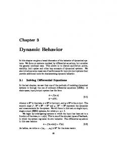
∂L d ∂L = +Υ dt ∂ q˙ ∂q is just a restatement of Newton’s law in generalized coordinates: d (momentum) = applied force. dt The motion of the individual particles can be recovered through application of equation (4.4). Example 4.1. Dynamics of a spherical pendulum Consider an idealized spherical pendulum as shown in Figure 4.1. The system consists of a point with mass m attached to a spherical joint by a massless rod of length l. We parameterize the configuration of the point mass by two scalars, θ and φ, which measure the angular displacement from the z- and x-axes, respectively. We wish to solve for the motion of the mass under the influence of gravity. 159

We begin by deriving the Lagrangian for the system. The position of the mass, relative to the origin at the base of the pendulum, is given by   l sin θ cos φ (4.6) r(θ, φ) =  l sin θ sin φ  . −l cos θ The kinetic energy is T =

) * 1 2 1 ml &r& ˙ 2 = ml2 θ˙2 + (1 − cos2 θ)φ˙ 2 2 2

and the potential energy is

V = −mgl cos θ, where g ≈ 9.8 m/sec2 is the gravitational constant. Thus, the Lagrangian is given by * ) 1 L(q, q) ˙ = ml2 θ˙2 + (1 − cos2 θ)φ˙ 2 + mgl cos θ, 2

where q = (θ, φ). Substituting L into Lagrange’s equations gives d ) 2 ˙* d ∂L = ml θ = ml2 θ¨ dt ∂ θ˙ dt ∂L = ml2 sin θ cos θ φ˙ 2 − mgl sin θ ∂θ

d ∂L d ) 2 2 ˙* = ml sin θφ = ml2 sin2 θ φ¨ + 2ml2 sin θ cos θ θ˙φ˙ dt ∂ φ˙ dt ∂L =0 ∂φ and the overall dynamics satisfy , , + + 2 ,+ , + ml 0 θ¨ −ml2 sin θ cos θ φ˙ 2 mgl sin θ = 0. + + 0 0 ml2 sin2 θ φ¨ 2ml2 sin θ cos θ θ˙φ˙

(4.7) Given the initial position and velocity of the point mass, equation (4.7) uniquely determines the subsequent motion of the system. The motion of the mass in R3 can be retrieved from equation (4.6).

2.2

Inertial properties of rigid bodies

To apply Lagrange’s equations to a robot, we must calculate the kinetic and potential energy of the robot links as a function of the joint angles 160

r B A g Figure 4.2: Coordinate frames for calculating the kinetic energy of a moving rigid body. and velocities. This, in turn, requires that we have a model for the mass distribution of the links. Since each link is a rigid body, its kinetic and potential energy can be defined in terms of its total mass and its moments of inertia about the center of mass. Let V ⊂ R3 be the volume occupied by a rigid body, and ρ(r), r ∈ V be the mass distribution of the body. If the object is made from a homogeneous material, then ρ(r) = ρ, a constant. The mass of the body is the volume integral of the mass density: m= ρ(r) dV. V

The center of mass of the body is the weighted average of the density: 1 ρ(r)r dV. r¯ = m V Consider the rigid object shown in Figure 4.2. We compute the kinetic energy as follows: fix the body frame at the mass center of the object and let (p, R) be a trajectory of the object relative to an inertial frame, where we have dropped all subscripts to simplify notation. Let r ∈ R3 be the coordinates of a body point relative to the body frame. The velocity of the point in the inertial frame is given by p˙ + R˙ r and the kinetic energy of the object is given by the following volume integral: 1 ˙ 2 dV. ρ(r)&p˙ + Rr& (4.8) T = 2 V

Expanding the product in the kinetic energy integral yields ) * 1 ˙ + &Rr& ˙ 2 dV. T = ρ(r) &p& ˙ 2 + 2p˙T Rr 2 V 161

The first term of the above expression gives the translational kinetic energy. The second term vanishes because the body frame is placed at the mass center of the object and ˙ ˙ dV = (p˙T R) ρ(r)r dV = 0. ρ(r)(p˙T R)r V

V

The last term can be simplified using properties of rotation and skewsymmetric matrices: 1 ˙ T (Rr) ˙ dV = 1 ρ(r)(Rr) ρ(r)(R. ω r)T (R. ω r) dV 2 V 2 V 1 = ρ(r)(. rω)T (. rω) dV 2 V /0 1 1 T T ρ(r). r r.dV ω =: ω T Iω, = ω 2 2 V

where ω ∈ R3 is the body R!×! defined by  Ixx I = Iyx Izx

angular velocity. The symmetric matrix I ∈ Ixy Iyy Izy

 Ixz Iyz  = − ρ(r). r2 dV V Izz

is called the inertia tensor of the object expressed in the body frame. It has entries Ixx = ρ(r)(y 2 + z 2 ) dx dy dz V Ixy = − ρ(r)(xy) dx dy dz, V

and the other entries are defined similarly. The total kinetic energy of the object can now be written as the sum of a translational component and a rotational component, 1 1 m&p& ˙ 2 + ω T Iω 2 + 2 , 1 b T mI 0 1 = (V ) V b =: (V b )T MV b , 0 I 2 2

T =

(4.9)

where V. b = g −1 g˙ ∈ se(3) is the body velocity, and M is called the generalized inertia matrix of the object, expressed in the body frame. The matrix M is symmetric and positive definite. Example 4.2. Generalized inertia matrix for a homogeneous bar Consider a homogeneous rectangular bar with mass m, length l, width w, and height h, as shown in Figure 4.3. The mass density of the bar is 162

z

y l

x h w

Figure 4.3: A homogeneous rectangular bar. m ρ = lwh . We attach a coordinate frame at the center of mass of the bar, with the coordinate axes aligned with the principal axes of the bar. The inertia tensor is evaluated using the previous formula:

Ixx

Ixy

-

- h/2 - w/2 - l/2 1 2 2 2 m 1 2 m 2 y + z 2 dx dy dz = y + z dV = lwh lwh V −h/2 −w/2 −l/2 / 0 2 m 1 1 3 m = lw h + lwh3 = (w2 + h2 ), lwh 12 12 - h/2 - w/2 - l/2 m m (xy) dx dy dz (xy) dV = − =− lwh −h/2 −w/2 −l/2 V lwh 0 - h/2 - w/2 / m 1 2 l/2 =− x y|−l/2 dy dz = 0. lwh −h/2 −w/2 2

The other entries are calculated in the same manner and we have:  m 2 2 0 0 12 (w + h ) m 2 2 . 0 0 I= 12 (l + h ) m 2 2 0 0 (l + w ) 12

The inertia tensor is diagonal by virtue of the fact that we coordinate axes with the principal axes of the box. The generalized inertia matrix is given by m 0 0 0 0 0 0 m 0 0 0 0 + , 0 0 m 0 0 0  mI 0 m 0 0 0 12 (w2 +h2 ) 0 0 M= =  2 m 2 0 I 0 0 0 0 0 12 (l +h ) 0 0 0

0

0

aligned the

2 m 2 12 (l +w )



 . 

The block diagonal structure of this matrix relies on attaching the body coordinate frame at center of mass (see Exercise 3).

163

l2 r2 θ2

l1

y r1

θ1

x Figure 4.4: Two-link planar manipulator.

2.3

Example: Dynamics of a two-link planar robot

To illustrate how Lagrange’s equations apply to a simple robotic system, consider the two-link planar manipulator shown in Figure 4.4. Model each link as a homogeneous rectangular bar with mass mi and moment of inertia tensor , + I$ =

Ixi 0 0 0 Iyi 0 0 0 Izi

relative to a frame attached at the center of mass of the link and aligned with the principle axes of the bar. Letting vi ∈ R3 be the translational velocity of the center of mass for the ith link and ωi ∈ R3 be the angular velocity, the kinetic energy of the manipulator is ˙ = 1 m1 &v1 &2 + 1 ω T I∞ ω∞ + ∞ *∈ &+∈ &∈ + ∞ ω T I∈ ω∈ . T (θ, θ) 2 2 1 ∈ ∈ ∈ Since the motion of the manipulator is restricted to the xy plane, &vi & is the magnitude of the xy velocity of the center of mass and ωi is a vector in the direction of the z-axis, with &ω1 & = θ˙1 and &ω2 & = θ˙1 + θ˙2 . We solve for the kinetic energy in terms of the generalized coordinates by using the kinematics of the mechanism. Let pi = (xi , yi , 0) denote the position of the ith center of mass. Letting r1 and r2 be the distance from the joints to the center of mass for each link, as shown in the figure, we have x ¯1 = r1 c1 y¯1 = r1 s1 x ¯2 = l1 c1 + r2 c12 y¯2 = l1 s1 + r2 s12

x ¯˙ 1 = −r1 s1 θ˙1 y¯˙ 1 = r1 c1 θ˙1 x ¯˙ 2 = −(l1 s1 + r2 s12 )θ˙1 − r2 s12 θ˙2 y¯˙ 2 = (l1 c1 + r2 c12 )θ˙1 + r2 c12 θ˙2 ,

where si = sin θi , sij = sin(θi + θj ), and similarly for ci and cij . The 164

kinetic energy becomes 1 1 1 1 m1 (x ¯˙ 21 + y¯˙ 12 ) + Iz1 θ˙12 + m2 (x ¯˙ 22 + y¯˙ 22 ) + Iz2 (θ˙1 + θ˙2 )2 2 2 2 2 + ,T + ,+ , ˙ ˙ 1 θ1 α + 2βc2 δ + βc2 θ1 , = δ + βc2 δ θ˙2 2 θ˙2 (4.10)

˙ = T (θ, θ)

where

α = Iz1 + Iz2 + m1 r12 + m2 (l12 + r22 ) β = m2 l1 r2

δ = Iz2 + m2 r22 . Finally, we can substitute the Lagrangian L = T into Lagrange’s equations to obtain (after some calculation) + α + 2βc2 δ + βc2

δ + βc2 δ

,+ , + θ¨1 −βs2 θ˙2 + βs2 θ˙1 θ¨2

,+ , + , −βs2 (θ˙1 + θ˙2 ) θ˙1 τ = 1 . τ2 0 θ˙2

(4.11) The first term in this equation represents the inertial forces due to acceleration of the joints, the second represents the Coriolis and centrifugal forces, and the right-hand side is the applied torques.

2.4

Newton-Euler equations for a rigid body

Lagrange’s equations provide a very general method for deriving the equations of motion for a mechanical system. However, implicit in the derivation of Lagrange’s equations is the assumption that the configuration space of the system can be parameterized by a subset of Rn , where n is the number of degrees of freedom of the system. For a rigid body with configuration g ∈ SE(3), Lagrange’s equations cannot be directly used to determine the equations of motion unless we choose a local parameterization for the configuration space (for example, using Euler angles to parameterize the orientation of the rigid body). Since all parameterizations of SE(3) are singular at some configuration, such a derivation can only hold locally. In this section, we give a global characterization of the dynamics of a rigid body subject to external forces and torques. We begin by reviewing the standard derivation of the equations of rigid body motion and then examine the dynamics in terms of twists and wrenches. Let g = (p, R) ∈ SE(3) be the configuration of a coordinate frame attached to the center of mass of a rigid body, relative to an inertial frame. Let f represent a force applied at the center of mass, with the coordinates of f specified relative to the inertial frame. The translational

165

equations of motion are given by Newton’s law, which can written in terms of the linear momentum mp˙ as f=

d (mp). ˙ dt

Since the mass of the rigid body is constant, the translational motion of the center of mass becomes f = m¨ p. (4.12) These equations are independent of the angular motion of the rigid body because we have used the center of mass to represent the position of the body. Similarly, the equations describing angular motion can be derived independently of the linear motion of the system. Consider the rotational motion of a rigid body about a point, subject to an externally applied torque τ . To derive the equations of motion, we equate the change in angular momentum to the applied torque. The angular momentum relative to an inertial frame is given by I ' ω ∫ , where I ' = RIRT is the instantaneous inertia tensor relative to the inertial frame and ω s is the spatial angular velocity. The angular equations of motion become τ=

, d ' ∫ (I ω ) = (RIRT ω ∫ ), dt ,-

where τ ∈ R3 is specified relative to the inertial frame. Expanding the right-hand side of this equation, we have T ∫ ˙ τ = RIRT ω˙ s + RIR ω + RI R˙ T ω ∫ ˙ T I ' ω ∫ + I ' RR˙ T ω ∫ = I ' ω˙ ∫ + RR

= I ' ω˙ ∫ + ω ∫ × I ' ω ∫ − I ' ω ∫ × ω ∫ ,

where the last equation follows by differentiating the identity RRT = I and using the definition of ω s . The last term of this equation is zero, and hence the dynamics are given by I ' ω˙ ∫ + ω ∫ × I ' ω ∫ = τ.

(4.13)

Equation (4.13) is called Euler’s equation. Equations (4.12) and (4.13) describe the dynamics of a rigid body in terms of a force and torque applied at the center of mass of the object. However, the coordinates of the force and torque vectors are not written relative to a body-fixed frame attached at the center of mass, but rather with respect to an inertial frame. Thus the pair (f, τ ) ∈ R6 is not the 166

wrench applied to the rigid body, as defined in Chapter 2, since the point of application is not the origin of the inertial coordinate frame. Similarly, the velocity pair (p, ˙ ω s ) does not correspond to the spatial or body velocity, since p˙ is not the correct expression for the linear velocity term in either body or spatial coordinates. In order to express the dynamics in terms of twists and wrenches, we rewrite Newton’s equation using the body velocity v b = RT p˙ and body force f b = RT f . Expanding the right-hand side of equation (4.12), d d b ˙ (mp) ˙ = (mRv b ) = Rmv˙ b + Rmv , dt dt and pre-multiplying by RT , the translational dynamics become mv˙ b + ω b × mv b = f b .

(4.14)

Equation (4.14) is Newton’s law written in body coordinates. Similarly, we can write Euler’s equation in terms of the body angular velocity ω b = RT ω s and the body torque τ b = RT τ . A straightforward computation shows that I ω˙ ) + ω ) × Iω ) = τ ) .

(4.15)

Equation (4.15) is Euler’s equation, written in body coordinates. Note that in body coordinates the inertia tensor is constant and hence we use I instead of I ' = RIRT . Combining equations (4.14) and (4.15) gives the equations of motion for a rigid body subject to an external wrench F applied at the center of mass and specified with respect to the body coordinate frame: + mI 0

0 I

,+

, + b , v˙ b ω × mv b + = Fb ω˙ b ω b × Iω b

(4.16)

This equation is called the Newton-Euler equation in body coordinates. It gives a global description of the equations of motion for a rigid body subject to an external wrench. Note that the linear and angular motions are coupled since the linear velocity in body coordinates depends on the current orientation. It is also possible to write the Newton-Euler equations relative to a spatial coordinate frame. This version is explored in Exercises 4 and 5. Once again the equations for linear and angular motion are coupled, so that the translational motion still depends on the rotational motion. In this book we shall always write the Newton-Euler equations in body coordinates, as in equation (4.16).

167

3

Dynamics of Open-Chain Manipulators

We now derive the equations of motion for an open-chain robot manipulator. We shall use the kinematics formulation presented in the previous chapter to write the Lagrangian for the robot in terms of the joint angles and joint velocities. Using this form of the dynamics, we explore several fundamental properties of robot manipulators which are of importance when proving the stability of robot control laws.

3.1

The Lagrangian for an open-chain robot

To calculate the kinetic energy of an open-chain robot manipulator with n joints, we sum the kinetic energy of each link. For this we define a coordinate frame, Li , attached to the center of mass of the ith link. Let b

b

gsli (θ) = eξ1 θ1 · · · eξi θi gsli (0) represent the configuration of the frame Li relative to the base frame of the robot, S. The body velocity of the center of mass of the ith link is given by b ˙ Vslb i = Jsl (θ)θ, i b b has the form where Jsl is the body Jacobian corresponding to gsli . Jsl i i

where

5 b Jsl (θ) = ξ1† i

···

ξi†

0 ···

ξj† = Ad−1 1 ξbj θj 2 ξj b e · · · eξi θi gsli (0)

6 0 , j≤i

is the jth instantaneous joint twist relative to the ith link frame. To b streamline notation, we write Jsl as Ji for the remainder of this section. i The kinetic energy of the ith link is ˙ ˙ = 1 (V b )T Mi V b = 1 θ˙T J T (θ)Mi Ji (θ)θ, Ti (θ, θ) sli i 2 sli 2

(4.17)

where Mi is the generalized inertia matrix for the ith link. Now the total kinetic energy can be written as ˙ = T (θ, θ)

n #

˙ =: 1 θ˙T M (θ)θ. ˙ Ti (θ, θ) 2 i=1

(4.18)

The matrix M (θ) ∈ Rn×n is the manipulator inertia matrix. In terms of the link Jacobians, Ji , the manipulator inertia matrix is defined as M (θ) =

n #

JiT (θ)Mi Ji (θ).

i=1

168

(4.19)

To complete our derivation of the Lagrangian, we must calculate the potential energy of the manipulator. Let hi (θ) be the height of the center of mass of the ith link (height is the component of the position of the center of mass opposite the direction of gravity). The potential energy for the ith link is Vi (θ) = mi ghi (θ), where mi is the mass of the ith link and g is the gravitational constant. The total potential energy is given by the sum of the contributions from each link: n n # # V (θ) = Vi (θ) = mi ghi (θ). i=1

i=1

Combining this with the kinetic energy, we have ˙ = L(θ, θ)

n ) # i=1

3.2

* ˙ − Vi (θ) = 1 θ˙T M (θ)θ˙ − V (θ). Ti (θ, θ) 2

Equations of motion for an open-chain manipulator

Let θ ∈ Rn be the joint angles for an open-chain manipulator. The Lagrangian is of the form ˙ = 1 θ˙T M (θ)θ˙ − V (θ), L(θ, θ) 2 where M (θ) is the manipulator inertia matrix and V (θ) is the potential energy due to gravity. It will be convenient to express the kinetic energy as a sum, n # ˙ =1 L(θ, θ) Mij (θ)θ˙i θ˙j − V (θ). (4.20) 2 i,j=1 The equations of motion are given by substituting into Lagrange’s equations, d ∂L ∂L − = Υi , dt ∂ θ˙i ∂θi where we let Υi represent the actuator torque and other nonconservative, generalized forces acting on the ith joint. Using equation (4.20), we have n n ) * # d # d ∂L = ( Mij θ˙j ) = Mij θ¨j + M˙ ij θ˙j dt ∂ θ˙i dt j=1 j=1 n 1 # ∂Mkj ˙ ˙ ∂V ∂L = . θk θj − ∂θi 2 ∂θi ∂θi j,k=1

169

The M˙ ij term can now be expanded in terms of partial derivatives to yield n #

Mij (θ)θ¨j +

j=1

0 n / # ∂V 1 ∂Mkj ˙ ˙ ∂Mij ˙ ˙ θj θk − θk θj + (θ) = Υi ∂θk 2 ∂θi ∂θi

j,k=1

i = 1, . . . , n.

Rearranging terms, we can write n # j=1

Mij (θ)θ¨j +

n #

j,k=1

∂V (θ) = Υi Γijk θ˙j θ˙k + ∂θi

i = 1, . . . , n,

(4.21)

where Γijk is given by Γijk

1 = 2

/

∂Mij (θ) ∂Mik (θ) ∂Mkj (θ) + − ∂θk ∂θj ∂θi

0

.

(4.22)

Equation (4.21) is a second-order differential equation in terms of the manipulator joint variables. It consists of four pieces: inertial forces, which depend on the acceleration of the joints; centrifugal and Coriolis forces, which are quadratic in the joint velocities; potential forces, of the ∂V ; and external forces, Υi . form ∂θ i The centrifugal and Coriolis terms arise because of the non-inertial frames which are implicit in the use of generalized coordinates. In the classical mechanics literature, one identifies terms of the form θ˙i θ˙j , i 0= j as Coriolis forces and terms of the form θ˙i2 as centrifugal forces. The functions Γijk are called the Christoffel symbols corresponding to the inertia matrix M (θ). The external forces can be divided into two components. Let τi repre˙ to be any other sent the applied torque at the joint and define −Ni (θ, θ) forces which act on the ith generalized coordinate, including conservative forces arising from a potential as well as frictional forces. (The reason for the negative sign in the definition of Ni will become apparent in a moment.) As an example, if the manipulator has viscous friction at the joints, then Ni would be defined as ˙ = − ∂V − β θ˙i , −Ni (θ, θ) ∂θi where β is the damping coefficient. Other forces acting on the manipulator, such as forces applied at the end-effector, can also be included by reflecting them to the joints (via the transpose of the appropriate Jacobian).

170

In order to put the equations of motion back into vector form, we ˙ ∈ Rn×n as define the matrix C(θ, θ) ˙ = Cij (θ, θ)

n #

k=1

n

1# Γijk θ˙k = 2

k=1

/

∂Mik ∂Mkj ∂Mij + − ∂θk ∂θj ∂θi

0

θ˙k .

(4.23) We call the matrix C the Coriolis matrix for the manipulator; the vector ˙ θ˙ gives the Coriolis and centrifugal force terms in the equations C(θ, θ) ˙ of motion. Note that there are other ways to define the matrix C(θ, θ) ˙ ˙ ˙ ˙ such that Cij (θ, θ)θj = Γijk θj θk . However, this particular choice has important properties which we shall later exploit. Equation (4.21) can now be rewritten as ˙ θ˙ + N (θ, θ) ˙ =τ M (θ)θ¨ + C(θ, θ)

(4.24)

˙ includes gravity where τ is the vector of actuator torques and N (θ, θ) terms and other forces which act at the joints. This is a second-order vector differential equation for the motion of the manipulator as a function of the applied joint torques. The matrices M and C, which summarize the inertial properties of the manipulator, have some important properties which we shall use in the sequel: Lemma 4.2. Structural properties of the robot equations of motion Equation (4.24) satisfies the following properties: 1. M (θ) is symmetric and positive definite. 2. M˙ − 2C ∈ Rn×n is a skew-symmetric matrix. Proof. Positive definiteness of the inertia matrix follows directly from its definition and the fact that the kinetic energy of the manipulator is zero only if the system is at rest. To show property 2, we calculate the components of the matrix M˙ − 2C: (M˙ − 2C)ij = M˙ ij (θ) − 2Cij (θ) n # ∂Mij ˙ ∂Mij ˙ ∂Mik ˙ ∂Mkj ˙ = θk − θk − θk + θk ∂θk ∂θk ∂θj ∂θi =

k=1 n #

k=1

∂Mik ˙ ∂Mkj ˙ θk − θk . ∂θi ∂θj

Switching i and j shows (M˙ − 2C)T = −(M˙ − 2C). Note that the skewsymmetry property depends upon the particular definition of C given in equation (4.23). 171

θ1 θ2

θ3

l1 L2

r1 l0

l2 L3

r2

L1 r0 S

Figure 4.5: Three-link, open-chain manipulator. Property 2 is often referred to as the passivity property since it implies, among other things, that in the absence of friction the net energy of the robot system is conserved (see Exercise 8). The passivity property is important in the proof of many control laws for robot manipulators. Example 4.3. Dynamics of a three-link manipulator To illustrate the formulation presented above, we calculate the dynamics of the three-link manipulator shown in Figure 4.5. The joint twists were computed in Chapter 3 (for the elbow manipulator) and are given by

ξ1 =

0 0  00  0 1

ξ2 =



0 −l0  0 −1 0 0

 

ξ3 =



0 −l0  l1 −1 0 0



.

To each link we attach a frame Li at the center of mass and aligned with principle inertia axes of the link, as shown in the figure: gsl1 (0)

! I = 0

)

0 0 r0

1

*"

gsl2 (0) =

!

I 0

)

0 r1 l0

1

*"

gsl3 (0) =

!

I 0

)

0 l1 +r2 l0

1

*"

.

With this choice of link frames, the link inertia matrices have the general form   mi 0 mi 0 mi   0 , M$ =   Ixi 0  Iyi 0 0

Izi

where mi is the mass of the object and Ixi , Iyi , and Izi are the moments of inertia about the x-, y-, and z-axes of the ith link frame.

172

To compute the manipulator inertia matrix, we first compute the body Jacobians corresponding to each link frame. A detailed, but straightforward, calculation yields  −r1 c2 0 0  0 0 0 000

b J1 = Jsl =  00 00 00  1 (0) 000 100

J3 =

b Jsl 3 (0)

The inertia matrix for  M11 M12 M (θ) = M21 M22 M31 M32

 −l

 =

0 0 0 −r1 0 −1 −s2 0 c2 0  0 0 l1 s 3 0 −r2 −l1 c3 −r2  −1 −1  . 0 0 0 0

b J2 = Jsl = 2 (0)

2 c2 −r2 c23

0 0 0 −s23 c23

0 0 0 0 0

the system is given by  M13 M23  = J1T M∞ J∞ + J∈T M∈ J∈ + J!T M! J! . M33

The components of M are given by

M11 = Iy2 s22 + Iy3 s223 + Iz1 + Iz2 c22 + Iz3 c223 + m2 r12 c22 + m3 (l1 c2 + r2 c23 )2 M12 = 0 M13 = 0 M21 = 0 M22 = Ix2 + Ix3 + m3 l12 + m2 r12 + m3 r22 + 2m3 l1 r2 c3 M23 = Ix3 + m3 r22 + m3 l1 r2 c3 M31 = 0 M32 = Ix3 + m3 r22 + m3 l1 r2 c3 M33 = Ix3 + m3 r22 . Note that several of the moments of inertia of the different links do not appear in this expression. This is because the limited degrees of freedom of the manipulator do not allow arbitrary rotations of each joint around each axis. The Coriolis and centrifugal forces are computed directly from the inertia matrix via the formula 0 n n / # 1 # ∂Mij ∂Mik ∂Mkj ˙ ˙ = Cij (θ, θ) Γijk θ˙k = + − θk . 2 ∂θk ∂θj ∂θi k=1

k=1

A very messy calculation shows that the nonzero values of Γijk are given 173

by: Γ112 = (Iy2 − Iz2 − m2 r12 )c2 s2 + (Iy3 − Iz3 )c23 s23 − m3 (l1 c2 + r2 c23 )(l1 s2 + r2 s23 ) Γ113 = (Iy3 − Iz3 )c23 s23 − m3 r2 s23 (l1 c2 + r2 c23 ) Γ121 = (Iy2 − Iz2 − m2 r12 )c2 s2 + (Iy3 − Iz3 )c23 s23 − m3 (l1 c2 + r2 c23 )(l1 s2 + r2 s23 ) Γ131 = (Iy3 − Iz3 )c23 s23 − m3 r2 s23 (l1 c2 + r2 c23 ) Γ211 = (Iz2 − Iy2 + m2 r12 )c2 s2 + (Iz3 − Iy3 )c23 s23 + m3 (l1 c2 + r2 c23 )(l1 s2 + r2 s23 ) Γ223 = −l1 m3 r2 s3 Γ232 = −l1 m3 r2 s3 Γ233 = −l1 m3 r2 s3 Γ311 = (Iz3 − Iy3 )c23 s23 + m3 r2 s23 (l1 c2 + r2 c23 ) Γ322 = l1 m3 r2 s3

Finally, we compute the effect of gravitational forces on the manipulator. These forces are written as ˙ = ∂V , N (θ, θ) ∂θ where V : Rn → R is the potential energy of the manipulator. For the three-link manipulator under consideration here, the potential energy is given by V (θ) = m1 gh1 (θ) + m2 gh2 (θ) + m3 gh3 (θ), where hi is the the height of the center of mass for the ith link. These can be found using the forward kinematics map b

b

gsli (θ) = eξ1 θ1 . . . eξi θi gsli (0), which gives h1 (θ) = r0 h2 (θ) = l0 − r1 sin θ2

h3 (θ) = l0 − l1 sin θ2 − r2 sin(θ2 + θ3 ). Substituting these expressions into the potential energy and taking the

174

derivative gives 

 0 ˙ = ∂V = −(m2 gr1 + m3 gl1 ) cos θ2 − m3 r2 cos(θ2 + θ3 )) . N (θ, θ) ∂θ −m3 gr2 cos(θ2 + θ3 )) This completes the derivation of the dynamics.

3.3

(4.25)

Robot dynamics and the product of exponentials formula

The formulas and properties given in the last section hold for any mechanical system with Lagrangian L = 12 θ˙T M (θ)θ˙ − V (θ). If the forward kinematics are specified using the product of exponentials formula, then it is possible to get more explicit formulas for the inertia and Coriolis matrices. In this section we derive these formulas, based on the treatments given by Brockett et al. [15] and Park et al. [87]. In addition to the tools introduced in Chapters 2 and 3, we will make use of one additional operation on twists. Recall, first, that in so(3) the cross product between two vectors ω1 , ω2 ∈ R3 yields a third vector, ω1 ×ω2 ∈ R3 . It can be shown by direct calculation that the cross product satisfies (ω1 × ω2 )∧ = ω .1 ω .2 − ω .2 ω .1 . By direct analogy, we define the Lie bracket on se(3) as [ξ.1 , ξ.2 ] = ξ.1 ξ.2 − ξ.2 ξ.1 .

A simple calculation verifies that the right-hand side of this equation has the form of a twist, and hence [ξ.1 , ξ.2 ] ∈ se(3). If ξ1 , ξ2 ∈ R6 represent the coordinates for two twists, we define the bracket operation [·, ·] : R6 × R6 → R6 as *∨ ) [ξ1 , ξ2 ] = ξ.1 ξ.2 − ξ.2 ξ.1 . (4.26) This is a generalization of the cross product on R3 to vectors in R6 . The following properties of the Lie bracket are also generalizations of properties of the cross product: = −[ξ2 , ξ1 ]

[ξ1 , [ξ2 , ξ3 ]] + [ξ2 , [ξ3 , ξ1 ]] + [ξ3 , [ξ1 , ξ2 ]] = 0. A more detailed (and abstract) description of the Lie bracket operation on se(3) is given in Appendix A. For this chapter we shall only need the formula given in equation (4.26) 175

We now define some additional notation which we use in the sequel. Let Aij ∈ R6×6 represent the adjoint transformation given by  −1  Ad(eξj+1 θj+1 · · · eξi θi ) i > j  (4.27) Aij = I i=j   0 i < j.

Using this notation, the jth column of the body Jacobian for the ith link is given by Adg−1 Aij ξj : sli

Ji (θ) = Adg−1

sli (0)

We combine Adg−1

sli (0)

5 Ai1 ξ1

···

Aii ξi

0 ···

6 0 .

with the link inertia matrix by defining the trans-

formed inertia matrix for the ith link: M'$ = AdT}−∞ M$ Ad}−∞ .

(4.28)

∫ $% (&)

∫ $% (&)

The matrix M'$ represents the inertia of the ith link reflected into the base frame of the manipulator. Using these definitions, we can obtain formulas for the inertial quantities which appear in the equation of motion. We state the results as a proposition. Proposition 4.3. Formulas for inertia and Coriolis matrices Using the notation defined above, the inertia and Coriolis matrices for an open-chain manipulator are given by Mij (θ) =

n #

l=max(i,j) n

1# Cij (θ) = 2

k=1

/

ξiT ATli M', A,| ξ|

∂Mij ∂Mik ∂Mkj + − ∂θk ∂θj ∂θi

0

(4.29) θ˙k ,

where ∂Mij = ∂θk

n #

l=max(i,j)

)

[Aki ξi , ξk ]T ATlk M', A,| ξ| * + ξiT ATli M', A,- [A-| ξ| , ξ- ] . (4.30)

This proposition shows that all of the dynamic attributes of the manipulator can be determined directly from the joint twists ξi , the link frames gsli (0) , and the link inertia matrices M$ . The matrices Aij are the only expressions in equations (4.29) and (4.30) which depend on the current configuration of the manipulator. 176

Proof. The only term which needs to be calculated in order to prove the proposition is ∂θ∂k (Alj ξj ). For i ≥ j, let gij ∈ SE(3) be the rigid transformation given by ; b b e−ξi θi . . . e−ξj+1 θj+1 i > j gij = I i = j, so that Aij = Adgij . Using this notation, if k is an integer such that i ≥ k ≥ j, then gij = gik gkj . We now proceed to calculate ∂θ∂k (Alj ξj ) for i ≥ k ≥ j: = / 0∨ < −1 ∨ ∂glj ∂ ∂ ) . −1 * ∂glj . −1 . ξ j glj + glj ξ j (Alj ξj ) = glj ξ j glj = ∂θk ∂θk ∂θk ∂θk *∨ ) −1 . −1 −1 ξ k glk = −gl,k ξ.k gkj ξ.j glj + glj ξ.j gkj *∨ ) −1 . −1 ξk = Adglk −ξ.k gkj ξ.j gkj + gkj ξ.j gkj = Alk [Akj ξj , ξk ].

For all other values of k, by direct calculation.

∂ ∂θk (Alj ξj )

is zero. The proposition now follows

Example 4.4. Dynamics of an idealized SCARA manipulator Consider the SCARA manipulator shown in Figure 4.6. The joint twists are given by 0 l   l +l  0 0

ξ1 =  00  0 1

1

0

ξ2 =  00  0 1

1

ξ3 = 

0 0 0 0 1

2



0

ξ4 =  10  . 0 0

Assuming that the link frames are initially aligned with the base frame and are located at the centers of mass of the links, the transformed link inertia matrices have the form , + , + ,+ ,+ I 0 mi I 0 I p.i mi I mi p.i ' = , M$ = −mi p.i I −. pi I 0 I 0 I

where pi is the location of the origin of the ith link frame relative to the base frame S. Given the joint twists ξi and transformed link inertias M'$ , the dynamics of the manipulator can be computed using the formulas in Proposition 4.3. This task is considerably simplified using the software described in Appendix B, so we omit a detailed computation and present only the final result. The inertia matrix M (θ) ∈ R4×4 is given by   α + β + 2γ cos θ2 β + γ cos θ2 δ 0  β + γ cos θ2 β δ 0  , M (θ) =   δ δ δ 0  0 0 0 m4 177

θ3 θ2 θ1

L2

L3

θ4

L1 L4 z S x

l0 y l1

l2

Figure 4.6: SCARA manipulator in its reference configuration. where

α = Iz1 + r12 m1 + l12 m2 + l12 m3 + l12 m4 β = Iz2 + Iz3 + Iz4 + l22 m3 + l22 m4 + m2 r22 γ = l1 l2 m3 + l1 l2 m4 + l1 m2 r2 δ = Iz3 + Iz4 .

The Coriolis matrix is given by  −γ sin θ2 θ˙2  γ sin θ2 θ˙1 ˙ = C(θ, θ)  0 0

 −γ sin θ2 (θ˙1 + θ˙2 ) 0 0 0 0 0 . 0 0 0 0 0 0

The only remaining term in the dynamics is the gravity term, which can be determined by inspection since only θ4 affects the potential energy of the manipulator. Hence,   0   ˙ =  0 . N (θ, θ)  0  m4 g Friction and other nonconservative forces can also be included in N .

178

4

Lyapunov Stability Theory

In this section we review the tools of Lyapunov stability theory. These tools will be used in the next section to analyze the stability properties of a robot controller. We present a survey of the results that we shall need in the sequel, with no proofs. The interested reader should consult a standard text, such as Vidyasagar [118] or Khalil [49], for details.

4.1

Basic definitions

Consider a dynamical system which satisfies x˙ = f (x, t)

x(t0 ) = x0

x ∈ Rn .

(4.31)

We will assume that f (x, t) satisfies the standard conditions for the existence and uniqueness of solutions. Such conditions are, for instance, that f (x, t) is Lipschitz continuous with respect to x, uniformly in t, and piecewise continuous in t. A point x∗ ∈ Rn is an equilibrium point of (4.31) if f (x∗ , t) ≡ 0. Intuitively and somewhat crudely speaking, we say an equilibrium point is locally stable if all solutions which start near x∗ (meaning that the initial conditions are in a neighborhood of x∗ ) remain near x∗ for all time. The equilibrium point x∗ is said to be locally asymptotically stable if x∗ is locally stable and, furthermore, all solutions starting near x∗ tend towards x∗ as t → ∞. We say somewhat crude because the time-varying nature of equation (4.31) introduces all kinds of additional subtleties. Nonetheless, it is intuitive that a pendulum has a locally stable equilibrium point when the pendulum is hanging straight down and an unstable equilibrium point when it is pointing straight up. If the pendulum is damped, the stable equilibrium point is locally asymptotically stable. By shifting the origin of the system, we may assume that the equilibrium point of interest occurs at x∗ = 0. If multiple equilibrium points exist, we will need to study the stability of each by appropriately shifting the origin. Definition 4.1. Stability in the sense of Lyapunov The equilibrium point x∗ = 0 of (4.31) is stable (in the sense of Lyapunov) at t = t0 if for any - > 0 there exists a δ(t0 , -) > 0 such that &x(t0 )& < δ

=⇒

&x(t)& < -,

∀t ≥ t0 .

(4.32)

Lyapunov stability is a very mild requirement on equilibrium points. In particular, it does not require that trajectories starting close to the origin tend to the origin asymptotically. Also, stability is defined at a time instant t0 . Uniform stability is a concept which guarantees that the equilibrium point is not losing stability. We insist that for a uniformly 179

stable equilibrium point x∗ , δ in the Definition 4.1 not be a function of t0 , so that equation (4.32) may hold for all t0 . Asymptotic stability is made precise in the following definition: Definition 4.2. Asymptotic stability An equilibrium point x∗ = 0 of (4.31) is asymptotically stable at t = t0 if 1. x∗ = 0 is stable, and 2. x∗ = 0 is locally attractive; i.e., there exists δ(t0 ) such that &x(t0 )& < δ

=⇒

lim x(t) = 0.

t→∞

(4.33)

As in the previous definition, asymptotic stability is defined at t0 . Uniform asymptotic stability requires: 1. x∗ = 0 is uniformly stable, and 2. x∗ = 0 is uniformly locally attractive; i.e., there exists δ independent of t0 for which equation (4.33) holds. Further, it is required that the convergence in equation (4.33) is uniform. Finally, we say that an equilibrium point is unstable if it is not stable. This is less of a tautology than it sounds and the reader should be sure he or she can negate the definition of stability in the sense of Lyapunov to get a definition of instability. In robotics, we are almost always interested in uniformly asymptotically stable equilibria. If we wish to move the robot to a point, we would like to actually converge to that point, not merely remain nearby. Figure 4.7 illustrates the difference between stability in the sense of Lyapunov and asymptotic stability. Definitions 4.1 and 4.2 are local definitions; they describe the behavior of a system near an equilibrium point. We say an equilibrium point x∗ is globally stable if it is stable for all initial conditions x0 ∈ Rn . Global stability is very desirable, but in many applications it can be difficult to achieve. We will concentrate on local stability theorems and indicate where it is possible to extend the results to the global case. Notions of uniformity are only important for time-varying systems. Thus, for time-invariant systems, stability implies uniform stability and asymptotic stability implies uniform asymptotic stability. It is important to note that the definitions of asymptotic stability do not quantify the rate of convergence. There is a strong form of stability which demands an exponential rate of convergence: Definition 4.3. Exponential stability, rate of convergence The equilibrium point x∗ = 0 is an exponentially stable equilibrium point of (4.31) if there exist constants m, α > 0 and - > 0 such that &x(t)& ≤ me−α(t−t0 ) &x(t0 )& 180

(4.34)

4

x˙

-4 -4

4 x (a) Stable in the sense of Lyapunov 4

0.4

x˙

x˙

-4 -4

-0.4 -0.4

4 x (b) Asymptotically stable

0.4 x (c) Unstable (saddle)

Figure 4.7: Phase portraits for stable and unstable equilibrium points. for all &x(t0 )& ≤ - and t ≥ t0 . The largest constant α which may be utilized in (4.34) is called the rate of convergence. Exponential stability is a strong form of stability; in particular, it implies uniform, asymptotic stability. Exponential convergence is important in applications because it can be shown to be robust to perturbations and is essential for the consideration of more advanced control algorithms, such as adaptive ones. A system is globally exponentially stable if the bound in equation (4.34) holds for all x0 ∈ Rn . Whenever possible, we shall strive to prove global, exponential stability.

4.2

The direct method of Lyapunov

Lyapunov’s direct method (also called the second method of Lyapunov) allows us to determine the stability of a system without explicitly integrating the differential equation (4.31). The method is a generalization of the idea that if there is some “measure of energy” in a system, then we can study the rate of change of the energy of the system to ascertain stability. To make this precise, we need to define exactly what one means 181

by a “measure of energy.” Let B% be a ball of size - around the origin, B% = {x ∈ Rn : &x& < -}. Definition 4.4. Locally positive definite functions (lpdf ) A continuous function V : Rn × R+ → R is a locally positive definite function if for some - > 0 and some continuous, strictly increasing function α : R+ → R, V (0, t) = 0

and V (x, t) ≥ α(&x&)

∀x ∈ B% , ∀t ≥ 0.

(4.35)

A locally positive definite function is locally like an energy function. Functions which are globally like energy functions are called positive definite functions: Definition 4.5. Positive definite functions (pdf ) A continuous function V : Rn × R+ → R is a positive definite function if it satisfies the conditions of Definition 4.4 and, additionally, α(p) → ∞ as p → ∞. To bound the energy function from above, we define decrescence as follows: Definition 4.6. Decrescent functions A continuous function V : Rn × R+ → R is decrescent if for some - > 0 and some continuous, strictly increasing function β : R+ → R, V (x, t) ≤ β(&x&)

∀x ∈ B% , ∀t ≥ 0

(4.36)

Using these definitions, the following theorem allows us to determine stability for a system by studying an appropriate energy function. Roughly, this theorem states that when V (x, t) is a locally positive definite function and V˙ (x, t) ≤ 0 then we can conclude stability of the equilibrium point. The time derivative of V is taken along the trajectories of the system: > ∂V ∂V > + f. V˙ > = ∂t ∂x x=f ˙ (x,t) In what follows, by V˙ we will mean V˙ |x=f ˙ (x,t) . Theorem 4.4. Basic theorem of Lyapunov Let V (x, t) be a non-negative function with derivative V˙ along the trajectories of the system. 1. If V (x, t) is locally positive definite and V˙ (x, t) ≤ 0 locally in x and for all t, then the origin of the system is locally stable (in the sense of Lyapunov). 2. If V (x, t) is locally positive definite and decrescent, and V˙ (x, t) ≤ 0 locally in x and for all t, then the origin of the system is uniformly locally stable (in the sense of Lyapunov). 182

Table 4.1: Summary of the basic theorem of Lyapunov.

1 2 3

Conditions on V (x, t) lpdf lpdf, decrescent lpdf, decrescent

Conditions on −V˙ (x, t) ≥ 0 locally ≥ 0 locally lpdf

4

pdf, decrescent

pdf

Conclusions Stable Uniformly stable Uniformly asymptotically stable Globally uniformly asymptotically stable

3. If V (x, t) is locally positive definite and decrescent, and −V˙ (x, t) is locally positive definite, then the origin of the system is uniformly locally asymptotically stable. 4. If V (x, t) is positive definite and decrescent, and −V˙ (x, t) is positive definite, then the origin of the system is globally uniformly asymptotically stable. The conditions in the theorem are summarized in Table 4.1. Theorem 4.4 gives sufficient conditions for the stability of the origin of a system. It does not, however, give a prescription for determining the Lyapunov function V (x, t). Since the theorem only gives sufficient conditions, the search for a Lyapunov function establishing stability of an equilibrium point could be arduous. However, it is a remarkable fact that the converse of Theorem 4.4 also exists: if an equilibrium point is stable, then there exists a function V (x, t) satisfying the conditions of the theorem. However, the utility of this and other converse theorems is limited by the lack of a computable technique for generating Lyapunov functions. Theorem 4.4 also stops short of giving explicit rates of convergence of solutions to the equilibrium. It may be modified to do so in the case of exponentially stable equilibria. Theorem 4.5. Exponential stability theorem x∗ = 0 is an exponentially stable equilibrium point of x˙ = f (x, t) if and only if there exists an - > 0 and a function V (x, t) which satisfies α1 &x&2 ≤ V (x, t) ≤ α2 &x&2 2 V˙ |x=f ˙ (x,t) ≤ −α3 &x& &

∂V (x, t)& ≤ α4 &x& ∂x

for some positive constants α1 , α2 , α3 , α4 , and &x& ≤ -. 183

The rate of convergence for a system satisfying the conditions of Theorem 4.5 can be determined from the proof of the theorem [102]. It can be shown that / 01/2 α2 α3 m≤ α≥ α1 2α2

are bounds in equation (4.34). The equilibrium point x∗ = 0 is globally exponentially stable if the bounds in Theorem 4.5 hold for all x.

4.3

The indirect method of Lyapunov

The indirect method of Lyapunov uses the linearization of a system to determine the local stability of the original system. Consider the system x˙ = f (x, t)

(4.37)

with f (0, t) = 0 for all t ≥ 0. Define

> ∂f (x, t) >> A(t) = ∂x >x=0

(4.38)

to be the Jacobian matrix of f (x, t) with respect to x, evaluated at the origin. It follows that for each fixed t, the remainder f1 (x, t) = f (x, t) − A(t)x approaches zero as x approaches zero. However, the remainder may not approach zero uniformly. For this to be true, we require the stronger condition that &f1 (x, t)& = 0. (4.39) lim sup &x& -x-→0 t≥0 If equation (4.39) holds, then the system z˙ = A(t)z

(4.40)

is referred to as the (uniform) linearization of equation (4.31) about the origin. When the linearization exists, its stability determines the local stability of the original nonlinear equation. Theorem 4.6. Stability by linearization Consider the system (4.37) and assume lim sup

-x-→0 t≥0

&f1 (x, t)& = 0. &x&

Further, let A(·) defined in equation (4.38) be bounded. If 0 is a uniformly asymptotically stable equilibrium point of (4.40) then it is a locally uniformly asymptotically stable equilibrium point of (4.37). 184

K M B q Figure 4.8: Damped harmonic oscillator. The preceding theorem requires uniform asymptotic stability of the linearized system to prove uniform asymptotic stability of the nonlinear system. Counterexamples to the theorem exist if the linearized system is not uniformly asymptotically stable. If the system (4.37) is time-invariant, then the indirect method says that if the eigenvalues of > ∂f (x) >> A= ∂x >x=0

are in the open left half complex plane, then the origin is asymptotically stable. This theorem proves that global uniform asymptotic stability of the linearization implies local uniform asymptotic stability of the original nonlinear system. The estimates provided by the proof of the theorem can be used to give a (conservative) bound on the domain of attraction of the origin. Systematic techniques for estimating the bounds on the regions of attraction of equilibrium points of nonlinear systems is an important area of research and involves searching for the “best” Lyapunov functions.

4.4

Examples

We now illustrate the use of the stability theorems given above on a few examples. Example 4.5. Linear harmonic oscillator Consider a damped harmonic oscillator, as shown in Figure 4.8. The dynamics of the system are given by the equation M q¨ + B q˙ + Kq = 0,

185

(4.41)

where M , B, and K are all positive quantities. As a state space equation we rewrite equation (4.41) as + , + , d q q˙ = . (4.42) −(K/M )q − (B/M )q˙ dt q˙ Define x = (q, q) ˙ as the state of the system. Since this system is a linear system, we can determine stability by examining the poles of the system. The Jacobian matrix for the system is + , 0 1 A= , −K/M −B/M

which has a characteristic equation

λ2 + (B/M )λ + (K/M ) = 0. The solutions of the characteristic equation are √ −B ± B 2 − 4KM λ= , 2M which always have negative real parts, and hence the system is (globally) exponentially stable. We now try to apply Lyapunov’s direct method to determine exponential stability. The “obvious” Lyapunov function to use in this context is the energy of the system, V (x, t) =

1 1 M q˙2 + Kq 2 . 2 2

(4.43)

Taking the derivative of V along trajectories of the system (4.41) gives V˙ = M q˙q¨ + Kq q˙ = −B q˙2 .

(4.44)

The function −V˙ is quadratic but not locally positive definite, since it does not depend on q, and hence we cannot conclude exponential stability. It is still possible to conclude asymptotic stability using Lasalle’s invariance principle (described in the next section), but this is obviously conservative since we already know that the system is exponentially stable. The reason that Lyapunov’s direct method fails is illustrated in Figure 4.9a, which shows the flow of the system superimposed with the level sets of the Lyapunov function. The level sets of the Lyapunov function become tangent to the flow when q˙ = 0, and hence it is not a valid Lyapunov function for determining exponential stability. To fix this problem, we skew the level sets slightly, so that the flow of the system crosses the level surfaces transversely. Define + ,T + ,+ , 1 q 1 1 K -M q V (x, t) = = qM ˙ q˙ + qKq + -qM ˙ q, -M M q˙ 2 q˙ 2 2 186

10

10

q˙

q˙

-10 -10

q

-10 -10

10

10

q

(a)

(b)

Figure 4.9: Flow of damped harmonic oscillator. The dashed lines are the level sets of the Lyapunov function defined by (a) the total energy and (b) a skewed modification of the energy. where - is a small positive constant such that V is still positive definite. The derivative of the Lyapunov function becomes V˙ = qM ˙ q¨ + qK q˙ + -M q˙2 + -qM q¨ = (−B + -M )q˙2 + -(−Kq 2 − Bq q) ˙ =−

+ ,T + -K q 1 q˙ 2 -B

,+ , q . B − -M q˙ 1 2 -B

The function V˙ can be made negative definite for - chosen sufficiently small (see Exercise 11) and hence we can conclude exponential stability. The level sets of this Lyapunov function are shown in Figure 4.9b. This same technique is used in the stability proofs for the robot control laws contained in the next section. Example 4.6. Nonlinear spring mass system with damper Consider a mechanical system consisting of a unit mass attached to a nonlinear spring with a velocity-dependent damper. If x1 stands for the position of the mass and x2 its velocity, then the equations describing the system are: x˙ 1 = x2 (4.45) x˙ 2 = −f (x2 ) − g(x1 ). Here f and g are smooth functions modeling the friction in the damper and restoring force of the spring, respectively. We will assume that f, g are both passive; that is, σf (σ) ≥ 0 σg(σ) ≥ 0

∀σ ∈ [−σ0 , σ0 ] ∀σ ∈ [−σ0 , σ0 ] 187

and equality is only achieved when σ = 0. The candidate for the Lyapunov function is - x1 x2 g(σ) dσ. V (x) = 2 + 2 0

The passivity of g guarantees that V (x) is a locally positive definite function. A short calculation verifies that V˙ (x) = −x2 f (x2 ) ≤ 0

when |x2 | ≤ σ0 .

This establishes the stability, but not the asymptotic stability of the origin. Actually, the origin is asymptotically stable, but this needs Lasalle’s principle, which is discussed in the next section.

4.5

Lasalle’s invariance principle

Lasalle’s theorem enables one to conclude asymptotic stability of an equilibrium point even when −V˙ (x, t) is not locally positive definite. However, it applies only to autonomous or periodic systems. We will deal with the autonomous case and begin by introducing a few more definitions. We denote the solution trajectories of the autonomous system x˙ = f (x)

(4.46)

as s(t, x0 , t0 ), which is the solution of equation (4.46) at time t starting from x0 at t0 . Definition 4.7. ω limit set The set S ⊂ Rn is the ω limit set of a trajectory s(·, x0 , t0 ) if for every y ∈ S, there exists a strictly increasing sequence of times tn such that s(tn , x0 , t0 ) → y as tn → ∞. Definition 4.8. Invariant set The set M ⊂ Rn is said to be an (positively) invariant set if for all y ∈ M and t0 ≥ 0, we have s(t, y, t0 ) ∈ M

∀t ≥ t0 .

It may be proved that the ω limit set of every trajectory is closed and invariant. We may now state Lasalle’s principle. Theorem 4.7. Lasalle’s principle Let V : Rn → R be a locally positive definite function such that on the compact set Ωc = {x ∈ Rn : V (x) ≤ c} we have V˙ (x) ≤ 0. Define S = {x ∈ Ωc : V˙ (x) = 0}. 188

As t → ∞, the trajectory tends to the largest invariant set inside S; i.e., its ω limit set is contained inside the largest invariant set in S. In particular, if S contains no invariant sets other than x = 0, then 0 is asymptotically stable. A global version of the preceding theorem may also be stated. An application of Lasalle’s principle is as follows: Example 4.7. Nonlinear spring mass system with damper Consider the same example as in equation (4.45), where we saw that with - x1 x2 g(σ) dσ, V (x) = 2 + 2 0 we obtained

V˙ (x) = −x2 f (x2 ).

Choosing c = min(V (−σ0 , 0), V (σ0 , 0)) so as to apply Lasalle’s principle, we see that V˙ (x) ≤ 0 for x ∈ Ωc := {x : V (x) ≤ c}. As a consequence of Lasalle’s principle, the trajectory enters the largest invariant set in Ωc ∩{x1 , x2 : V˙ = 0} = Ωc ∩{x1 , 0}. To obtain the largest invariant set in this region, note that x2 (t) ≡ 0

=⇒

x1 (t) ≡ x10

=⇒

x˙ 2 (t) = 0 = −f (0) − g(x10 ),

where x10 is some constant. Consequently, we have that g(x10 ) = 0

=⇒

x10 = 0.

Thus, the largest invariant set inside Ωc ∩ {x1 , x2 : V˙ = 0} is the origin and, by Lasalle’s principle, the origin is locally asymptotically stable. There is a version of Lasalle’s theorem which holds for periodic systems as well. However, there are no significant generalizations for nonperiodic systems and this restricts the utility of Lasalle’s principle in applications.

5

Position Control and Trajectory Tracking

In this section, we consider the position control problem for robot manipulators: given a desired trajectory, how should the joint torques be chosen so that the manipulator follows that trajectory. We would like to choose a control strategy which is robust with respect to initial condition errors, sensor noise, and modeling errors. We ignore the problems of actuator dynamics, and assume that we can command arbitrary torques which are exerted at the joints. 189

5.1

Problem description

We are given a description of the dynamics of a robot manipulator in the form of the equation ˙ θ˙ + N (θ, θ) ˙ = τ, M (θ)θ¨ + C(θ, θ)

(4.47)

where θ ∈ Rn is the set of configuration variables for the robot and τ ∈ Rn denotes the torques applied at the joints. We are also given a joint trajectory θd (·) which we wish to track. For simplicity, we assume that θd is specified for all time and that it is at least twice differentiable. ˙ If we have a perfect model of the robot and θ(0) = θd (0), θ(0) = θ˙d (0), then we may solve our problem by choosing τ = M (θd )θ¨d + C(θd , θ˙d )θ˙d + N (θd , θ˙d ). Since both θ and θd satisfy the same differential equation and have the same initial conditions, it follows from the uniqueness of the solutions of differential equations that θ(t) = θd (t) for all t ≥ 0. This an example of an open-loop control law: the current state of the robot is not used in choosing the control inputs. Unfortunately, this strategy is not very robust. If θ(0) 0= θd (0), then the open-loop control law will never correct for this error. This is clearly undesirable, since we almost never know the current position of a robot exactly. Furthermore, we have no guarantee that if our starting configuration is near the desired initial configuration that the trajectory of the robot will stay near the desired trajectory for all time. For this reason, we introduce feedback into our control law. This feedback must be chosen such that the actual robot trajectory converges to the desired trajectory. In particular, if our trajectory is a single setpoint, the closed-loop system should be asymptotically stable about the desired setpoint. There are several approaches for designing stable robot control laws. Using the structural properties of robot dynamics, we will be able to prove stability of these control laws for all robots having those properties. Hence, we do not need to design control laws for a specific robot; as long as we show that stability of a particular control algorithm requires only those properties given in Lemma 4.2 on page 171, then our control law will work for general open-chain robot manipulators. Of course, the performance of a given control law depends heavily on the particular manipulator, and hence the control laws presented here should only be used as a starting point for synthesizing a feedback compensator.

5.2

Computed torque

Consider the following refinement of the open-loop control law presented above: given the current position and velocity of the manipulator, cancel 190

all nonlinearities and apply exactly the torque needed to overcome the inertia of the actuator, ˙ θ˙ + N (θ, θ). ˙ τ = M (θ)θ¨d + C(θ, θ) Substituting this control law into the dynamic equations of the manipulator, we see that M (θ)θ¨ = M (θ)θ¨d , and since M (θ) is uniformly positive definite in θ, we have θ¨ = θ¨d .

(4.48)

Hence, if the initial position and velocity of the manipulator matches the desired position and velocity, the manipulator will follow the desired trajectory. As before, this control law will not correct for any initial condition errors which are present. The tracking properties of the control law can be improved by adding state feedback. The linearity of equation (4.48) suggests the following control law: ) * ˙ θ˙ + N (θ, θ) ˙ τ = M (θ) θ¨d − Kv e˙ − Kp e + C(θ, θ) (4.49) where e = θ − θd , and Kv and Kp are constant gain matrices. When substituted into equation (4.47), the error dynamics can be written as: M (θ) (¨ e + Kv e˙ + Kp e) = 0. Since M (θ) is always positive definite, we have e¨ + Kv e˙ + Kp e = 0.

(4.50)

This is a linear differential equation which governs the error between the actual and desired trajectories. Equation (4.49) is called the computed torque control law. The computed torque control law consists of two components. We can write equation (4.49) as τ = M (θ)θ¨d + C θ˙ + N + M (θ) (−Kv e˙ − Kp e) . @A B ? ? @A B τff

τfb

The term τff is the feedforward component. It provides the amount of torque necessary to drive the system along its nominal path. The term τfb is the feedback component. It provides correction torques to reduce any errors in the trajectory of the manipulator. Since the error equation (4.50) is linear, it is easy to choose Kv and Kp so that the overall system is stable and e → 0 exponentially as t → ∞. 191

Moreover, we can choose Kv and Kp such that we get independent exponentially stable systems (by choosing Kp and Kv diagonal). The following proposition gives one set of conditions under which the computed torque control law (4.49) results in exponential tracking. Proposition 4.8. Stability of the computed torque control law If Kp , Kv ∈ Rn×n are positive definite, symmetric matrices, then the control law (4.49) applied to the system (4.47) results in exponential trajectory tracking. Proof. The error dynamics can be written as a first-order linear system: + , + ,+ , d e 0 I e = . −Kp −Kv e˙ dt e˙ ? @A B A

It suffices to show that each of the eigenvalues of A has negative real part. Let λ ∈ C be an eigenvalue of A with corresponding eigenvector v = (v1 , v2 ) ∈ C2n , v 0= 0. Then, + , + ,+ , + , v 0 I v1 v2 λ 1 = = . v2 −Kp −Kv v2 −Kp v1 − Kv v2

It follows that if λ = 0 then v = 0, and hence λ = 0 is not an eigenvalue of A. Further, if λ 0= 0, then v2 = 0 implies that v1 = 0. Thus, v1 , v2 0= 0 and we may assume without loss of generality that &v1 & = 1. Using this, we write λ2 = v1∗ λ2 v1 = v1∗ λv2 = v1∗ (−Kp v1 − Kv v2 ) = −v1∗ Kp v1 − λv1∗ Kv v1 ,

where ∗ denotes complex conjugate transpose. Since α = v1∗ Kp v1 > 0 and β = v1∗ Kv v1 > 0, we have λ2 + αλ + β = 0

α, β > 0

and hence the real part of λ is negative. The power of the computed torque control law is that it converts a nonlinear dynamical system into a linear one, allowing the use of any of a number of linear control synthesis tools. This is an example of a more general technique known as feedback linearization, where a nonlinear system is rendered linear via full-state nonlinear feedback. One disadvantage of using feedback linearization is that it can be demanding (in terms of computation time and input magnitudes) to use feedback to globally convert a nonlinear system into a single linear system. For robot manipulators, unboundedness of the inputs is rarely a problem since the inertia matrix of the system is bounded and hence the control torques which must be exerted always remain bounded. In addition, experimental results show that the computed torque controller has very good performance characteristics and it is becoming increasingly popular. 192

5.3

PD control

Another approach to controller synthesis for nonlinear systems is to design a linear controller based on the linearization of the system about an operating point. Since the linearization of a system locally determines the stability of the full system, this class of controllers is guaranteed to be locally stable. In many situations, it is possible to prove global stability for a linear controller by explicit construction of a Lyapunov function. An example of this design methodology is a proportional plus derivative (PD) control law for a robot manipulator. In its simplest form, a PD control law has the form τ = −Kv e˙ − Kp e,

(4.51)

where Kv and Kp are positive definite matrices and e = θ − θd . Since this control law has no feedforward term, it can never achieve exact tracking for non-trivial trajectories. A common modification is to add an integral term to eliminate steady-state errors. This introduces additional complications since care must be taken to maintain stability and avoid integrator windup. Before adding a feedforward term, we first show that the PD controller gives asymptotic setpoint stabilization. Proposition 4.9. If θ˙d ≡ 0 and Kv , Kp > 0, the control law (4.51) applied to the system (4.47) renders the equilibrium point θ = θd globally asymptotically stable. Proof. For θd ≡ 0, the closed-loop system is ˙ θ˙ + Kv θ˙ + Kp (θ − θd ) = 0. M (θ)θ¨ + C(θ, θ)

(4.52)

Without loss of generality, we assume that θd = 0 (if not, redefine θ' = θ − θd ). We choose the total energy of the system as our Lyapunov function, ˙ = 1 θ˙T M (θ)θ˙ + 1 θT Kp θ. V (θ, θ) 2 2 The function V is (globally) positive definite and decresent. Evaluating V˙ along trajectories of (4.52), ˙ = θ˙T M θ¨ + 1 θ˙T M˙ θ˙ + θ˙T Kp θ V˙ (θ, θ) 2 1 T ˙ = −θ˙ Kv θ˙ + θ˙T (M˙ − 2C)θ, 2 and since M˙ − 2C is skew-symmetric, we have ˙ V˙ = −θ˙T Kv θ. 193

Although Kv is positive definite, the function V˙ is only negative semidefinite, since V˙ = 0 for θ˙ = 0 and θ 0= 0. Hence from Lyapunov’s basic theorem, we can concluded only stability of the equilibrium point. To check for asymptotic stability, we appeal to Lasalle’s principle. The set S for which V˙ ≡ 0 is given by ˙ : θ˙ ≡ 0}. S = {(θ, θ) To find the largest invariant set contained in S, we substitute θ˙ ≡ 0 into the closed loop equations 4.52. This gives Kp θ = 0 (recalling that θd = 0) and since Kp is positive definite, it follows that the largest invariant set contained within S is the single point θ = 0. Hence, the equilibrium point θ = 0 is asymptotically stable. Since we are primarily interested in tracking, we consider a modified version of the PD control law: ˙ θ˙d + N (θ, θ) ˙ − Kv e˙ − Kp e τ = M (θ)θ¨d + C(θ, θ)

(4.53)

We call this controller the augmented PD control law. Note that the sec˙ θ. ˙ ond term in equation (4.53) is different from the Coriolis term C(θ, θ) The reason for this difference is found in the proof of the following theorem. Proposition 4.10. Stability of the PD control law The control law (4.53) applied to the system (4.47) results in exponential trajectory tracking if Kv , Kp > 0. Proof. The closed-loop system is ˙ e˙ + Kv e˙ + Kp e = 0. M (θ)¨ e + C(θ, θ)

(4.54)

As in the proof of the previous proposition, using the energy of the system as a Lyapunov function does not allow us to conclude exponential stability because V˙ is only negative semi-definite. Furthermore, since the system is time-varying (due to the θd (·) terms), we cannot apply Lasalle’s principle. To show exponential stability, we adopt the same approach as with the spring mass system of the previous section. Namely, we skew the level sets of the energy function by choosing the Lyapunov function candidate V (e, e, ˙ t) =

1 T 1 e˙ M (θ)e˙ + eT Kp e + -eT M (θ)e, ˙ 2 2 194

which is positive definite for - sufficiently small since M (θ) > 0 and Kp > 0. Evaluating V˙ along trajectories of (4.54): 1 2 1 V˙ = e˙ T M e¨ + e˙ T M˙ e˙ + e˙ T Kp e + -e˙ T M e˙ + -eT M e¨ + M˙ e˙ 2 1 2 1 T = −e˙ (Kv − -M )e˙ + e˙ T (M˙ −2C)e˙ + -eT −Kp e−Kv e−C ˙ e+ ˙ M˙ e˙ 2 1 T = −e˙ (Kv − -M )e˙ − -eT Kp e + -eT (−Kv + M˙ )e˙ 2 Choosing - > 0 sufficiently small insures that V˙ is negative definite (see Exercise 11) and hence the system is exponentially stable using Theorem 4.5. If θ˙d ≡ 0, i.e., we wish to stabilize a point, the control law (4.53) simplifies to the original PD control law (4.51). We also note that asymptotic tracking requires exact cancellation of friction and gravity forces and relies on accurate models of these quantities as well as the manipulator inertia matrix. In practice, errors in modeling will result in errors in tracking. A further difficulty in using the PD control law is choosing the gains Kp and Kv . The linearization of the system about a given operating point θ0 gives error dynamics of the form M (θ0 )¨ e + Kv e˙ + Kp e = 0. Since this is a linear system, it is possible to choose Kv and Kp to achieve a given performance specification using linear control theory. However, if we are tracking a trajectory, then there is no guarantee that we will remain near θ0 and the chosen gains may not be appropriate. In practice, one can usually get reasonable results by choosing the gains based on the linearization about an equilibrium point in the middle of the robot’s workspace.

5.4

Workspace control

Suppose we are given a path gd (t) ∈ SE(3) which represents the desired configuration of the end-effector as a function of time. One way to move the manipulator along this path is to solve the inverse kinematics problem at each instant in time and generate a desired joint angle trajectory θd (t) ∈ Q such that g(θd (t)) = gd (t). The methods of the previous sections can then be used to generate a feedback controller which follows this path. There are several disadvantages to solving the feedback control problem in this manner. Since solving the inverse kinematics problem is a time-consuming task, systems in which gd is specified in real-time must 195

use powerful computers to compute θd at a rate suitable for control. Furthermore, it may be difficult to choose the feedback gains in joint space in a meaningful way, since the original task was given in terms of the end-effector trajectory. For example, a joint-space, computed torque controller with diagonal gain matrices (Kp and Kv ) will generate a decoupled response in joint space, resulting in straight line trajectories in θ if the setpoint of the manipulator is changed. However, due to the nonlinear nature of the kinematics, this will not generate a straight line trajectory in SE(3). For many tasks, this type of behavior is undesirable. To overcome these disadvantages, we consider formulating the problem directly in end-effector coordinates. In doing so, we will eliminate the need to solve the inverse kinematics and also generate controllers whose gains have a more direct connection with the task performance. However, in order to use the tools developed in Section 4, we must choose a set of local coordinates for SE(3), such as parameterizing orientation via Euler angles. This limits the usefulness of the technique somewhat, although for many practical applications this limitation is of no consequence. This approach to writing controllers is referred to as workspace control, since x represents the configuration of the end-effector in the workspace of the manipulator. Let f : Q → Rp be a smooth and invertible mapping between the joint variables θ ∈ Q and the workspace variables x ∈ Rp . In particular, this requires that n = p so that the number of degrees of freedom of the robot equals the number of workspace variables x. We allow for the possibility that p < 6, in which case the workspace variables may only give a partial parameterization of SE(3). An example of this situation is the SCARA robot, for which the position of the end-effector and its orientation with respect to the z-axis form a natural set of coordinates for specifying a task. The dynamics of the manipulator in joint space has the form ˙ θ˙ + N (θ, θ) ˙ = τ, M (θ)θ¨ + C(θ, θ) where τ is the vector of joint torques and M , C, and N describe the dynamic parameters of the system, as before. We can rewrite the dynamics in terms of x ∈ Rp by using the Jacobian of the mapping f : θ 7→ x, x˙ = J(θ)θ˙

J(θ) =

∂f . ∂θ

Note that J is the Jacobian of the mapping f : Q → Rp and not the manipulator Jacobian. Under the assumption that f is smooth and invertible, we can write θ˙ = J −1 x˙

and

d θ¨ = J −1 x ¨ + (J −1 )x. ˙ dt 196

We can now substitute these expressions into the manipulator dynamics and pre-multiply by J −T := (J −1 )T to obtain J

−T

M (θ)J

−1

/

x ¨+ J

−T

0 d −1 −1 −T ˙ C(θ, θ)J + J M (θ) (J ) x˙ dt ˙ = J −T τ. + J −T N (θ, θ)

We can write this in a more familiar form by defining ˜ = J −T M J −1 M 0 / d 1 −1 2 −T −1 ˜ C=J CJ + M J dt ˜ = J −T N N F = J −T τ, in which case the dynamics become ˙ x˙ + N ˙ = F. ˜ (θ)¨ ˜ θ) ˜ (θ, θ) M x + C(θ,

(4.55)

This equation represents the dynamics in terms of the workspace coordi˜ , C, ˜ and N ˜ the effective nates x and the robot configuration θ. We call M parameters of the system. They represent the dynamics of the system as viewed from the workspace variables. Since f is locally invertible, we can in fact eliminate θ from these equations, and we see that equation (4.55) is nothing more than Lagrange’s equations relative to the generalized coordinates x. However, since for most robots we measure θ directly and compute x via the forward kinematics, it is convenient to leave the θ dependence explicit. Equation (4.55) has the same basic structure as the dynamics for an open-chain manipulator written in joint coordinates. In order to exploit this structure in our control laws, we must verify that some of the properties which we used in proving stability of controllers are also satisfied. The following lemma verifies that this is indeed the case. Lemma 4.11. Structural properties of the workspace dynamics Equation (4.55) satisfies the following properties: ˜ (θ) is symmetric and positive definite. 1. M ˜˙ − 2C˜ ∈ Rn×n is a skew-symmetric matrix. 2. M Proof. Since J is an invertible matrix, property 1 follows from its defini˜˙ − 2C: ˜ tion. To show property 2, we calculate the M ˜ J −1 − J −T M ˜ d (J −1 ). ˜˙ − 2C˜ = J −T (M ˜˙ − 2C)J ˜ −1 + d (J −T )M M dt dt 197

A direct calculation shows that this matrix is indeed skew-symmetric. These two properties allow us to immediately extend the control laws in the previous section to workspace coordinates. For example, the computed torque control law becomes ˙ x˙ + N (θ, θ) ˙ ˜ (θ) (¨ F =M xd − Kv e˙ − Kp e) + C(θ, θ) τ = J T F,

where xd is the desired workspace trajectory and e = x − xd is the workspace error. The proof of stability for this control law is identical to that given previously. Namely, using the fact that M (θ) is positive definite, we can write the workspace error dynamics as e¨ + Kv e˙ + Kp e = 0 which is again a linear differential equation whose stability can be verified directly. The PD control law can be similarly extended to workspace coordinates. The advantage of writing the control law in this fashion is that the matrices Kv and Kp now specify the gains directly in workspace coordinates. This simplifies the task of choosing the gains that are needed to accomplish a specific task. Furthermore, it eliminates the need to solve for the inverse mapping f −1 in order to control the robot. Instead, we only have to calculate the Jacobian matrix for f and its (matrix) inverse. Notice that when the manipulator approaches a singular configuration ˜ gets very large. This relative to the coordinates x, the effective inertia M is an indication that it is difficult to move in some directions and hence large forces produce very little motion. It is important to note that this singularity is strictly a function of our choice of parameterization. Such singularities never appear in the joint space of the robot. Example 4.8. Comparison of joint space and workspace controllers To illustrate some of the differences between implementing a controller in joint space versus workspace, we consider the control of a planar two degree of freedom robot. We take as our workspace variables the xy position of the end-effector. Figure 4.10 shows the step response of a computed torque control law written in joint coordinates. Note that the trajectory of the end-effector, shown on the right, follows a curved path. The time response of the joint trajectories is a classical linear response for an underdamped mechanical system. Figure 4.11 shows the step response of a computed torque control law written in workspace coordinates. Now the trajectory of the end-effector, including the overshoot, follows a straight line in the workspace and a curved line in the joint space.

198

Trajectory in joint coordinates

Trajectory in Cartesian coordinates

2

2

1.5

1.5

overshoot

1

1

desired

0.5

desired overshoot

start

0.5

start

0

0

-0.5 -0.5

0

0.5

1

1.5

-0.5 -0.5

2

Joint space trajectory versus time

0

0.5

1

1.5

2

Work space trajectory versus time

2

2 θ1

1

x y

1

θ2

0

0 0

1

2

0

1

2

Figure 4.10: Step response of a joint space, computed torque controller.

Trajectory in joint coordinates

Trajectory in Cartesian coordinates

2

2

desired 1.5

overshoot

1.5

1 0.5

1

overshoot

desired

start

0.5

start

0

0

-0.5 -0.5

0

0.5

1

1.5

-0.5 -0.5

2

Joint space trajectory versus time

0

0.5

1

1.5

2

Work space trajectory versus time

2

2 θ1

1

x y

1

θ2

0

0 0

1

2

0

1

2

Figure 4.11: Step response of a workspace, computed torque controller.

199

6

Control of Constrained Manipulators

In this short section, we provide a brief treatment of the control of constrained manipulators. A more thorough development is given in Chapter 6.

6.1

Dynamics of constrained systems

Consider a problem in which we wish to move the tip of a robot along a surface and apply a force against that surface. For simplicity, we assume the surface is frictionless, although the analysis presented here can be readily extended to the more general case. We suppose that the surface we wish to move along can be described by a set of independent, smooth constraints hj (θ1 , . . . , θn ) = 0 j = 1, . . . , k, (4.56) and that there exists a smooth, injective map f : Rn−k → Rn such that hj (f1 (φ), · · · , fn (φ)) = 0.

(4.57)

That is, φ ∈ Rn−k parameterizes the allowable motion on the surface and θ = f (φ) corresponds to a configuration in which the robot is in contact with the surface. The control task is to follow a given trajectory φd (t) while applying a force against the surface. Since the surface is represented in joint space as the level set of the map h(θ) = 0, the normal vectors to this surface are given by the span of the gradients of ∇hi . (Since the surface is n − k dimensional, the dimension of the space of normal vectors is k.) Any torques of the form # τN = λj ∇hj (θ) (4.58) correspond to normal forces applied against the surface. In the absence of friction, the work done by these torques is given by # # / ∂hi 0 θ˙ τN · θ˙ = λi ∇hi · θ˙ = λi ∂θ # d = λi (h(θ)) = 0. dt

Hence the normal forces do no work on the system and therefore cause no motion in the system. We assume that a desired normal force, specified by λ1 (t), . . . , λk (t), is given as part of the task description. If the robot remains in contact with the surface, as desired, then the dynamics of the manipulator can be written in terms of φ. Differentiating

200

θ = f (φ), we have ∂f ˙ φ θ˙ = ∂φ / 0 ∂f ¨ d ∂f ˙ ¨ φ+ φ. θ= ∂φ dt ∂φ

(4.59)

These equations can be substituted into the robot equations of motion, ˙ θ˙ + N (θ, θ) ˙ =τ M (θ)θ¨ + C(θ, θ) to yield / / 00 ∂f ¨ d ∂f ∂f ˙ ˙ = τ, M (θ) φ + C(θ, θ) + M (θ) φ˙ + N (θ, θ) ∂φ ∂φ dt ∂φ

(4.60)

where we have left M , C, and N in terms of θ to simplify notation. Equation (4.60) can be made symmetric by multiplying both sides by ∂f T ∂φ .

Letting J =

∂f ∂φ (φ),

we define

˜ (φ) = J T M (f (φ))J M ) * ˙ = J T C(f (φ), J φ)J ˙ + M (f (φ))J˙ ˜ φ) C(φ,

˙ = J T N (f (φ), J φ) ˙ ˜ (φ, φ) N

(4.61)

F = J T τ. Using these definitions, the projected equations of motion can be written as ˙ φ˙ + N ˙ = F. ˜ (φ)φ¨ + C(φ, ˜ φ) ˜ (φ, φ) M (4.62) This equation has the same form as the equation for an unconstrained manipulator. We shall show in Chapter 6 that equation (4.62) also satisfies the properties in Lemma 4.2. This is not particularly surprising since the coordinates φ were chosen to be a set of generalized coordinates under the assumption that the robot maintains contact with the surface. It is important to keep in mind that equation (4.62) represents the dynamics of the system only along the surface given by the level sets h(θ) = 0. By pre-multiplying by J T , we have eliminated the information about the forces of constraint. For many applications, we are interested in regulating the forces of constraint and hence we must use the full equations of motion given in equation (4.60).

6.2

Control of constrained manipulators

The control task for a constrained robot system is to simultaneously regulate the position of the system along the constraint surface and regulate the forces of the system applied against this surface. In terms of analyzing stability, it is enough to analyze only the motion along the surface, 201

since no movement occurs perpendicular to the surface. Of course, implicit in this point of view is that we maintain contact with the surface. If the manipulator is not physically constrained, this may require that we regulate the forces so as to insure that we are always pushing against the surface and never pulling away from it. In this section we show how to extend the computed torque formalism presented earlier to regulate the position and force of the manipulator. We give only a sketch of the approach, leaving a more detailed discussion until Chapter 6, where we shall see that hybrid position/force control is just one example of the more general problem of controlling single and multiple robots interacting with each other and their environment. We take as given a path on the constraint surface, specified by φd (t), and a normal force to be applied against the surface, specified by the Lagrange multipliers λ1 (t), . . . , λk (t) as in equation (4.58). Since we are interested in regulating the force applied against the constraint, it is important to insure that the position portion of the controller does not push against the constraint. Define τφ = M (θ)

∂f ¨ (φd − Kv e˙ φ − Kp eφ ) ∂φ / / 00 ∂f d ∂f ˙ ˙ + C(θ, θ) + M (θ) φ˙ + N (θ, θ), ∂φ dt ∂φ

where eφ = φ − φd . This is the torque required to move the manipulator along the surface while applying no force against the surface. In other words, if we apply τ = τφ and remove the constraint completely, the manipulator will follow the correct path, as if the constraint were present. To apply the appropriate normal forces, we simply add τN as defined in equation (4.58) to τφ . Since τN is in the normal direction to the constraint, it does not affect the position portion of the controller. Of course, this requires that the constraint surface actually be present to resist the normal forces applied to it. The complete control law is given by τ = τφ +

k #

λi (t)∇hi

(4.63)

i=1

where τφ is given above. We defer the analysis and proof of convergence for this control law until Chapter 6. As in the previous control laws, the force control law presented here relies on accurate models of the robot and the surface. In particular, we note that the applied normal force does not use feedback to correct for model error, sensor noise, or other non-ideal situations.

202

θ2 n

s

α

θ1 q l

Figure 4.12: Planar manipulator moving in a slot.

6.3

Example: A planar manipulator moving in a slot

As a simple example of a constrained manipulator, consider the control of a two degree of freedom, planar manipulator whose end-effector is forced to lie in a slot, as shown in Figure 4.12. This system resembles a slidercrank mechanism, except that we are allowed to apply torques on both revolute joints, allowing us to control both the motion of the slider as well as the force applied against the slot. This example is easily adapted to a robot pushing against a wall, in which case the forces against the slot must always be pointed in a preferred direction. We take the slot to be a straight line passing through the point q = (l, 0) and making an angle α with respect to the x-axis of the base frame. The vector normal to the direction of the slot is given by + , sin α n= , − cos α and the slot can be described as the set of all points p ∈ R2 such that (p − q) · n = 0. The constraint on the manipulator is obtained by requiring that the position of the end-effector remain in the slot. Letting p(θ) ∈ R2 represent the position of the tool frame, this constraint becomes / + ,0 + , l sin α h(θ) = p(θ) − · = 0. 0 − cos α Substituting the forward kinematics of the manipulator yields h(θ) = (l1 cos θ1 + l2 cos(θ1 + θ2 ) − l) sin α

− (l1 sin θ1 + l2 sin(θ1 + θ2 )) cos α = −l1 sin(θ1 − α) − l2 sin(θ1 + θ2 − α) − l sin α. 203

The gradient of the constraint, which gives the direction of the normal force, is given by + , −l1 cos(θ1 − α) − l2 cos(θ1 + θ2 − α) ∇h(θ) = . −l2 cos(θ1 + θ2 − α) Note that this is the direction of the normal force in joint coordinates. That is, joint torques applied in this direction will cause no motion, only forces against the side of the slot. To parameterize the allowable motion along the slot, we let s ∈ R represent the position along the slot, with s = 0 denoting the point q = (l, 0). Finding a function f (s) such that h(f (s)) = 0 involves solving the inverse kinematics of the manipulator: given the position along the slot, we must find joint angles which achieve that position. If the end of the manipulator is at a position s along the slot, then the xy coordinates of the end-effector are x(s) = l + s cos α y(s) = s sin α. Solving the inverse kinematics (see Chapter 3, Section 3) and assuming the elbow down solution, we have  ) * * ) 2 s +2ls cos α+l2 +l12 −l22 s sin α + , tan−1 l+s + cos−1 2l √s2 +2ls cos α+l 2 cos α 1 θ (s)   f (s) = 1 = )2 2 2 * . 2 θ2 (s) −1 l1 +l2 −s −2ls cos α−l π + cos 2l1 l2 The Jacobian of the mapping is given by  −(s+l cos α)(s2 +2ls cos α+l2 −l2 +l2 )

1 2 r 2 2 cos α+l2 +l2 1 −l2 )  2l1 (s2 +2ls cos α+l2 ) 32 1− (s +2ls 2 2 2

J =

4l1 (s +2ls cos α+l )

+

√ 2 2 22(s+l cos α) 2 2 2 2 4l1 l2 −(s +2ls cos α+l −l1 −l2 )

l sin α

s2 +l2 +2ls cos α

  

(after some simplification). This matrix can now be used to compute the equations of motion and derive an appropriate control law. In particular, the computed torque controller has the form ) * ˙ + M (θ)J˙ s˙ + λn, τ = M (θ)J (¨ sd − Kv e˙ s − Kp es ) + C(θ, θ)J

where es = s − sd ; λ is the desired force against the slot; Kv , Kp ∈ R are the gain and damping factors; and M and C are the generalized inertial and Coriolis matrices. The inertial parameters were calculated in Section 2.3 and are given by , + 1 + , − 2 βs2 θ˙2 − 12 βs2 (θ˙1 + θ˙2 ) α+βc2 δ+ 12 βc2 ˙ C(θ, θ) = 1 M (θ) = , ˙ δ δ+ 12 βc2 0 2 βs2 θ1 204

where

α = Iz1 + Iz2 + m1 r12 + m2 (l12 + r22 ) β = m2 l 1 l 2

δ = Iz2 + m2 r22 . It is perhaps surprising that such a simple problem can have such an unwieldy solution. The difficulty is that we have cast the entire problem into the joint space of the manipulator, where the constraint θ = f (s) is a very complex looking curve. A better way of deriving the equations of motion for this system is to rewrite the dynamics of the system in terms of workspace variables which describe the position of the end-effector (see Exercise 12). Once written in this way, the constraint that the end of the manipulator remain in the slot is a very simple one. This is the basic approach used in Chapter 6, where we present a general framework which incorporates this example and many other constrained manipulation systems.

205

7

Summary

The following are the key concepts covered in this chapter: 1. The equations of motion for a mechanical system with Lagrangian L = T (q, q) ˙ − V (q) satisfies Lagrange’s equations: ∂L d ∂L − = Υi , dt ∂ q˙i ∂qi where q ∈ Rn is a set of generalized coordinates for the system and Υ ∈ Rn represents the vector of generalized external forces. 2. The equations of motion for a rigid body with configuration g(t) ∈ SE(3) are given by the Newton-Euler equations: + ,+ , + b , mI 0 v˙ b ω × mv b + b = F b, 0 I ω˙ b ω × Iω b where m is the mass of the body, I is the inertia tensor, and V b = (v b , ω b ) and F b represent the instantaneous body velocity and applied body wrench. 3. The equations of motion for an open-chain robot manipulator can be written as ˙ θ˙ + N (θ, θ) ˙ =τ M (θ)θ¨ + C(θ, θ) where θ ∈ Rn is the set of joint variables for the robot and τ ∈ Rn is the set of actuator forces applied at the joints. The dynamics of a robot manipulator satisfy the following properties: (a) M (θ) is symmetric and positive definite. (b) M˙ − 2C ∈ Rn×n is a skew-symmetric matrix. 4. An equilibrium point x∗ for the system x˙ = f (x, t) is locally asymptotically stable if all solutions which start near x∗ approach x∗ as t → ∞. Stability can be checked using the direct method of Lyapunov, by finding a locally positive definite function V (x, t) ≥ 0 such that −V˙ (x, t) is a locally positive definite function along trajectories of the system. In situations in which −V˙ is only positive semi-definite, Lasalle’s invariance principle can be used to check asymptotic stability. Alternatively, the indirect method of Lyapunov can be employed by examining the linearization of the system, if it exists. Global exponential stability of the linearization implies local exponential stability of the full nonlinear system.

206

5. Using the form and structure of the robot dynamics, several control laws can be shown to track arbitrary trajectories. Two of the most common are the computed torque control law, ˙ θ˙ + N (θ, θ), ˙ τ = M (θ)(θ¨d + Kv e˙ + Kp e) + C(θ, θ) and an augmented PD control law, ˙ θ˙d + N (θ, θ) ˙ + Kv e˙ + Kp e. τ = M (θ)θ¨d + C(θ, θ) Both of these controllers result in exponential trajectory tracking of a given joint space trajectory. Workspace versions of these control laws can also be derived, allowing end-effector trajectories to be tracked without solving the inverse kinematics problem. Stability of these controllers can be verified using Lyapunov stability.

8

Bibliography

The Lagrangian formulation of dynamics is classical; a good treatment can be found in Rosenberg [99] or Pars [89]. Its application to the dynamics of a robot manipulator can be found in most standard textbooks on robotics, for example [2, 21, 35, 52, 110]. The geometric formulation of the equations of motion for kinematic chains presented in Section 3.3 is based on the recent work of Brockett, Stokes, and Park [15, 87]. This is closely related to the spatial operator algebra formulation of Rodriguez, Jain, and Kreutz-Delgado [45, 98], in which the tree-like nature of the system is more fully exploited in computing inertial properties of the system. The literature on control of robot manipulators is vast. An excellent treatment, covering many of the different approaches to robot control, is given by Spong and Vidyasagar [110]. The collection [109] also provides a good survey of recent research in this area. The modified PD control law presented in Section 5 was originally formulated by Koditschek [51]. For a survey of manipulator control using exact linearization techniques, see Kreutz [53]. The use of skew terms in Lyapunov functions to prove exponential stability for PD controllers has been pointed out, for example, by Wen and Bayard [120].

207

9

Exercises 1. Derive the equations of motion for the systems shown below. y l1 x

θ1 θ2 l2 m1 g

θ m2 g (a)

(b)

(a) Pendulum on a wire: an idealized planar pendulum whose pivot is free to slide along a horizontal wire. Assume that the top of the pendulum can move freely on the wire (no friction). (b) Double pendulum: two masses connected together by massless links and revolute joints. 2. Compute the inertia tensor for the objects shown below. r c

h

b

a (a) Ellipsoid

(b) Cylinder

3. Transformation of the generalized inertia matrix Show that under a change of body coordinate frame from B to C, the generalized inertia matrix for a rigid body is given by + , T mI mRbc p.bc Rbc T Mc = Adgbc Mb Adgbc = , T T −mRbc p.bc Rbc Rbc (I − m. p2bc )Rbc

where gbc denotes the rigid motion taking C to B, and Mb and Mc are the generalized inertia matrices expressed in frame B and frame C.

4. Show that Euler’s equation written in spatial coordinates is given by I ' ω˙ ∫ + ω ∫ × I ' ω ∫ = τ, 208

where I ' = RIRT and τ is the torque applied to the center of mass of the rigid body, written in spatial coordinates. 5. Calculate the Newton-Euler equations in spatial coordinates. 6. Show that it is possible to choose M and C such that the NewtonEuler equations can be written as M V˙ b + C(g, g)V ˙ b = F b, where M > 0 and M˙ − 2C is a skew-symmetric matrix. 7. Verify that the equations of motion for a planar, two-link manipulator, as given in equation (4.11), satisfy the properties of Lemma 4.2. 8. Passivity of robot dynamics Let H = T + V be the total energy for a rigid robot. Show that if M˙ − 2C is skew-symmetric, then energy is conserved, i.e., H˙ = θ˙ · τ . 9. Show that the workspace version of the PD control law results in exponential trajectory tracking. 10. Show that the control law ˙ θ˙d + λe) + N (θ, θ) ˙ + Kv e˙ + Kp e τ = M (θ)(θ¨d + λe) ˙ + C(θ, θ)( results in exponential trajectory tracking when λ ∈ R is positive and Kv , Kp ∈ Rn×n are positive definite [107]. 11. Show that the matrix +

-A -B T

-B C + -D

,

is positive definite if A and C are symmetric, positive definite, and - > 0 is chosen sufficiently small. 12. Hybrid control using workspace coordinates Consider the constrained manipulation problem described in Section 6.3. Let pst (θ) ∈ R2 be the coordinates of the end-effector and let w = p(θ) represent a set of workspace coordinates for the system. (a) Compute the matrix J(θ) which is used to convert the joint space dynamics into workspace dynamics (as in Section 5.4). (b) Compute the constraint function in terms of the workspace variables and find a parameterization f : R → R2 which maps the slot position to the workspace coordinates. Let K(s) represent the Jacobian of the mapping w = f (s). 209

(c) Write the dynamics of the constrained system in terms of ω and its derivatives, the dynamic parameters of the unconstrained system, and the matrices J(θ) and K(s). (d) Verify that the equations of motion derived in step (c) are the same as the equations of motion derived in Section 6.3. In ˜ (s) are the particular, show that τN and the inertia matrix M same in both cases.

210