systems it is possible for some computers to be heavily ... schemes for multi-user jobs in heterogeneous distributed systems. ...... Computers and Digital Tech-.
Dynamic Multi-User Load Balancing in Distributed Systems Satish Penmatsa£and Anthony T. ChronopoulosÝ The University of Texas at San Antonio Dept. of Computer Science One UTSA Circle, San Antonio, Texas 78249, USA spenmats, atc�@cs.utsa.edu Abstract In this paper, we review two existing static load balancing schemes based on M/M/1 queues. We then use these schemes to propose two dynamic load balancing schemes for multi-user (multi-class) jobs in heterogeneous distributed systems. These two dynamic load balancing schemes differ in their objective. One tries to minimize the expected response time of the entire system while the other tries to minimize the expected response time of the individual users. The performance of the dynamic schemes is compared with that of the static schemes using simulations with various loads and parameters. The results show that, at low communication overheads, the dynamic schemes show superior performance over the static schemes. But as the overheads increase, the dynamic schemes (as expected) yield similar performance to that of the static schemes.
1. Introduction Load balancing is one of the most important problems in attaining high performance in distributed systems which may consist of many heterogeneous resources connected via one or more communication networks. In these distributed systems it is possible for some computers to be heavily loaded while others are lightly loaded. This situation can lead to a poor system performance. The goal of load balancing is to improve the performance of the system by balancing the loads among the computers. There are many studies on static load balancing for single-user (single-class) and multi-user (multi-class) jobs £ Student Member IEEE Ý Senior Member IEEE
This work was supported in part by National Science Foundation under grant CCR-0312323. c 2007 IEEE. 1-4244-0910-1/07/$20.00
that provide system-optimal solution [9, 13, 14] and references there-in. Individual-optimal policies based on Wardrop equilibrium when the number of users are infinite are studied in [9]. User-optimal (class-optimal) policies based on Nash equilibrium are studied in [6, 12] for finite number of users. Many dynamic load balancing policies exist [7, 10, 1, 2, 3, 4, 11, 15] and references there-in. Most of these dynamic policies are for single-class jobs and their main objective is to minimize the expected response time of the entire system. So, individual users jobs may get delayed which may not be acceptable in current distributed systems, where the users have requirements for fast job execution. In this paper, we propose two dynamic load balancing schemes for multi-user jobs in heterogeneous distributed systems. The computers in the distributed system are connected by a communication network. We review two existing static load balancing schemes and extend them to dynamic schemes. These two existing load balancing schemes differ in their objective. (i) The first scheme, GOS [9] tries to minimize the expected response time of the entire system. (ii) The second scheme, NCOOPC tries to minimize the expected response time of the individual users (to provide a user-optimal solution). We base our dynamic schemes on the static schemes (i) and (ii). The performance of the dynamic schemes is compared with that of the static schemes using simulations with various system conditions. The results show that, at low communication overheads, the dynamic schemes show superior performance over the static schemes. But as the overheads increase, the dynamic schemes as expected tend to perform similar to that of the static schemes. The paper is organized as follows. In Section 2, we present the system model. In Section 3, we review the two static load balancing schemes based on which the dynamic schemes are proposed in Section 4. The performance of the dynamic schemes is compared with that of the static schemes using simulations in Section 5. Conclusions are drawn and future work is stated in Section 6.
2. System Model
� : Mean utilization of the communication network � (� � �� �� ).
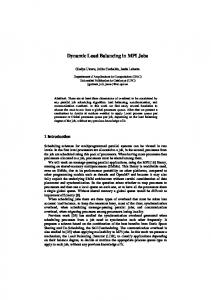
We consider a distributed system model as shown in Figure 1. The system has ‘ ’ nodes connected by a communication network. The nodes and the communication network are modeled as M/M/1 queuing systems (���� Poisson arrivals and exponentially distributed processing times) [8]. Jobs arriving at each node may belong to ‘�’ different users. We use the terminology and notations similar to [12] and also introduce some additional notations as follows:
�
: Mean utilization of the communication network � excluding user � traffic (� � � �� ��� � ).
We assume that the jobs arriving from various users to a node differ in their arrival rates but have the same execution time. j βi
�� : Mean interarrival time of a user � job to node �. �� : Mean job arrival rate of user � to node � (��
��
).
node 1
node 2
�
node n node i
� : Total job arrival rate of user � . � ��
Processor
j φi
j x ri
��
� : Total job arrival rate of the system. � � � �
j x ir
Communication Network
Figure 1. Distributed System Model
�� : Mean service time of a job at node �. � : Mean service rate of node � ( �
��
).
� : Job processing rate (load) of user � at node �.
� � � � �� � � � � � �� �� , is the vector of loads at node � from users �� � � � � �.
� � � � � � � � � �� , is the load vector of all nodes �� � � � � (from all users �� � � � � �).
� � � � �� � � � � � �� �� , is the vector of loads of user to nodes �� � � � � .
�
�� : Job flow rate of user � from node � to node �. � : Job traffic through the network of user � . �
� ��
� ��
��
� = �� � �� � � � � � �� �� ; �
�
�
�.
�� : Mean number of jobs of user � at node �. � : Number of jobs of user instant.
� at node � at a given
� : Time period for the exchange of job count of each user by all the nodes. � � : Time period for the exchange of arrival rates of each user by all the nodes.
� : Mean communication time for sending or receiving a job from one node to another for any user.
3. Static Load Balancing In this section, we study two static load balancing schemes based on which two dynamic load balancing schemes are derived in the next section. These static schemes are also used for comparison in Section 5 to evaluate the performance of the dynamic schemes. The following are the assumptions for static load balancing, similar to [9]. A job arriving at node � may be either processed at node � or transferred to another node � for remote processing through the communication network. A job can only be transferred at most once. The decision of transferring a job does not depend on the state of the system and hence is static in nature. If a node � sends (receives) jobs to (from) node �, node � does not send (receive) jobs to (from) node �. For each user � , nodes are classified into Active source nodes (�� ), Idle source nodes (� ), Neutral nodes (� ) and Sink nodes (� ) as in [9]. The expected response time of a user � job processed at node � is denoted by �� � � �. The expected communication delay of a user � job from node � to node � is denoted by � ��� and it is assumed to be independent of the sourcedestination pair ��� �� but it may depend on the total traffic through the network, �. Based on our assumptions on the node and the network models in the previous section, we have the following relations for the node and communication delays [8]:
�� � � �
� � �
�
� ��
�� �
(1)
� ���
�� � �
�
� ��
�� �
�
�� �
�
�
�
�
��
(2)
��� ������ � � �� ��� � ��� � This static load balancing scheme is proposed and studied in [9]. It minimizes the expected job response time of the entire system. The problem of minimizing the entire system expected job response time is expressed as
� ��� � � � � � ����
�� �� � �
�
�
� ��
�
�
�
(3)
�
��
�
�
� � ��
�
�� � � � � �
(4)
�� � � � � � �� � � � � �
�
(5)
The above nonlinear optimization problem is solved by using the Kuhn-Tucker theorem and an algorithm to compute the optimal loads ( � ) is presented in [9]. The user � marginal node delay �� � � � and marginal communication delay � ��� are defined as
�� � � �
� � �
� ���
� ��
� � �
��
� �
� �
� � � � � �
� � � ��� �
��
�
�
�� � �
�
� ��
�
� ��
�� �� �� ��
(6)
(7)
where �� ��� � � � denotes the mean number of user jobs in node � and �� �� ��� denotes the mean number of user jobs in the communication network.
��� ������ ��� ��� ��� � �� � �� �� ���� ��� �������� Here, we review a static load balancing scheme whose goal is to minimize the expected job response time of the individual users (���� to obtain a user-optimal solution). This problem is formulated, taking into account the users mean node delays and the mean communication delays, as a noncooperative game among the users. This noncooperative approach for multi-user job allocation with communication and pricing (NASHPC) for grid systems was studied in [12]. The grid users try to minimize the expected cost of their own jobs. The problem was formulated as a noncooperative game among the grid users and the Nash equilibrium provides the solution. Here, we are interested in the load balancing algorithm for multiuser jobs without pricing. Therefore, we take � � (� �� � � � � );
� � ��
� �� � � � � � ���� �
� � � � � ��
�
subject to the constraints:
�
�� � � � � , � �� � � � � �); and � = �� = 1 in equation (6) of [12]. Then, we obtain a noncooperative load balancing game where the users try to minimize the expected response time of their own jobs. Each user � (� �� � � � � �) must find her workload ( � ) �� � � � � ) such that the exthat is assigned to node � (� pected response time of her own jobs (� � �) is minimized, where
�� = 1 (�
��
(8)
��
� � �
�
� ��
�� �
�� � � � ��
��
�� �
�
(9)
Each user minimizes her own response time independently of the others and they all eventually reach an equilibrium. We use the concept of Nash equilibrium [5] as the solution of this noncooperative game. At the equilibrium, a user cannot decrease her own response time any further by changing her decision alone. � � � � � � � � � � is called the load balThe vector
�� � � � � �) and the vector ancing strategy of user � (�
� � � � � � � � � � � is called the strategy profile of the load balancing game. The strategy of user � depends on the load balancing strategies of the other users. At the Nash equilibrium, a user � cannot further decrease her expected response time by choosing a different load balancing strategy when the other users strategies are fixed. The equilibrium strategy profile can be found when each user’s load balancing strategy is a best response to the other users strategies. The best response for user � , is a solution to the following optimization problem:
�� � � �
(10)
subject to the following constraints for the existence of a feasible strategy profile:
� � ��
�
�
�
��
�
�
�
� � �
�
�� � � � �
�
(11)
� �
(12)
�� � � � �
(13)
We define the following functions for each user � :
� � � � �
� � � � � �� � � � �
� ���
� �� � ���� ��
� � � � � � ��� � �
�� � �
�
�
� � � �� �� � � � � ��
�
� � �� � ��
� �� �� � � ��
(14)
(15)
�� � � � � � � � �
�
� � � ��
�
��
��
if � if
��
(16)
��
The solution to the optimization problem in (10) is similar to the one in [12] where the �� � � � and � ��� in Theorem 3.1 of [12] are replaced by the above equations � � � � � and � ��� (equations (14) and (15)). The ! is used as the Lagrange multiplier which categorizes the nodes for each user � into sets of Active source nodes (�� �! �), Idle source nodes (� �! �), Neutral nodes (� �! �) and Sink nodes (� �! �). The �� �! � denotes the network traffic of user � because of jobs sent by the set of Active and Idle source nodes as determined by ! and �� �! � is the network traffic of user � because of jobs received by the set of Sink nodes as determined by ! [12]. The best response of user � (� �� � � � � �) can be determined using a BEST-RESPONSE algorithm similar to that in [12] where the �� , � and ��� � in [12] are replaced by
� � , � and �� � � above. The optimal loads of each user � (� �� � � � � �) ���� the equilibrium solution, can be ob-
tained using an iterative algorithm where each user updates her strategies (by computing her best response) periodically by fixing the other users startegies. The users form a virtual ring topology to communicate and iteratively apply the BEST-RESPONSE algorithm to compute the Nash equilibrium. This is implemented in the following algorithm. NCOOPC distributed load balancing algorithm: �� � � � � � in the ring performs the folEach user � , � lowing steps in each iteration: 1. Receive the current strategies of all the other users from the left neighbor. 2. If the message is a termination message, then pass the termination message to the right neighbor and EXIT. 3. Update the strategies ( ) by calling the BESTRESPONSE. 4. Calculate � (equation (9)) and update the error norm. 5. Send the updated strategies and the error norm to the right neighbor. At the equilibrium solution, the � � � � �� � of each user at
all the nodes are balanced.
4. Dynamic Load Balancing Kameda ����"� [16] proposed and studied dynamic load balancing algorithms for single user job streams based on M/M/1 queues in heterogeneous distributed systems. We follow a similar approach to extend GOS and NCOOPC to
dynamic schemes. In this section, we propose these two distributed dynamic load balancing schemes for multi-user jobs. A distributed dynamic scheme has three components: 1) an information policy used to disseminate load information among nodes, 2) a transfer policy that determines whether job transfer activities are needed by a computer, and 3) a location policy that determines which nodes are suitable to participate in load exchanges. The dynamic schemes which we propose use the number of jobs waiting in the queue to be processed (queue length) as the state information. The information policy is a periodic policy where the state information is exchanged between the nodes every � time units. When a job arrives at a node, the transfer policy component determines whether the job should be processed locally or should be transferred to another node for processing. If the job is eligible for transfer, the location policy component determines the destination node for remote processing. In the following we discuss the dynamic load balancing schemes.
���� ���� �� ������ � � �� ��� � ���� � The goal of DGOS is to balance the workload among the nodes dynamically in order to obtain a system-wide optimization ���� to minimize the expected response time of all the jobs over the entire system. We base the derivation of DGOS on the static GOS of Section 3. We use the following proposition to express the marginal node delay of a user � job at node � (�� � � � in equation (6)) in terms of the mean service time at node � (�� ) and the mean number of jobs of user � at node � (�� , � �� � � � � �). Proposition 4.1 The user � marginal node delay in equation (6) can be expressed in terms of �� and �� (� �� � � � � �) as
�� � � �
�� ��
�� � �
��
� �
�
Proof: In the Appendix. Rewriting equation (7) in terms of �, we have
� ���
�
�� � ��� �
���
(17)
¾ (18)
We next express �� �� of Proposition 4.1 and � �� from equation (18), which use the mean estimates of the system parameters, in terms of instantaneous variables. ¼ Let � denote the utilization of the network at a given instant. Replacing �� ’s, the mean number of jobs of users
at node � by � ’s and �, the mean utilization of the network ¼ by � , in equations (17) and (18), we obtain (for user � )
�� ��
�� �
� �
��
�
�� � � �� �
��
(19)
� ��
(20)
� �
¼
¼
The above relations are used as the estimates of the user
� marginal virtual node delay at node � and user � marginal communication delay. Whereas GOS tries to balance the marginal node delays of each user at all the nodes statically, DGOS will be derived to balance the marginal virtual node delays of each user at all the nodes dynamically. For a user # job arriving at node � that is eligible to transfer, each potential destination node � (� �� � � � � � � �) is compared with node �. Definition 4.1 If ��� � � �� , then node � is said to be more heavily loaded than node � for a user # job. We use the following proposition to determine a light node � relative to node � for a user # job, in the DGOS algorithm discussed below. Proposition 4.2 If node � is more heavily loaded than node � � � � , where
� for a user # job, then, � �
��
��
��
� �
��
�
�� ��
� �
�
��
� �
�
�
�� ���
� �
� � (21)
¾ Proof: In the Appendix. We next describe the components of dynamic GOS (information policy, transfer policy and location policy). 1) Information policy: Each node � (� �� � � � � ) broadcasts the number of jobs of user � (� �� � � � � �) in its queue (���� � ’s) to all the other nodes. This state information exchange is done every � time units. 2) Transfer policy: A threshold policy is used to determine whether an arriving job should be processed locally or should be transferred to another node. A user � job arriving at node � will be eligible to transfer when the number of jobs of user � at node � is greater than some threshold denoted by $� . Otherwise the job will be processed locally. The thresholds $� at a node � (� �� � � � � ) for each user � (� �� � � � � �) are calculated as follows: Each node � broadcasts its arrival rates (�� ) to all the � . Using other nodes every � � time units where � � this information all the nodes execute GOS to determine the optimal loads ( � ). These optimal loads are then converted (using Littles law [8], see proof of Proposition 4.1) into optimal number of jobs of user � that can be present at node �
(thresholds $� ). The above calculated thresholds are fixed for an interval of � � time units. This time interval can be adjusted based on the frequency of variation of the arrival rates at each node. 3) Location policy: The destination node for a user # job �� � � � � �) at node � that is eligible to transfer is de(# termined based on the state information that is exchanged from the information policy. First, a node with the shortest marginal virtual delay for a user # job (lightest node) is determined. Next, it is determined whether the arriving job should be transferred based on the transfers the user # job already had. (i) A node with the lightest load for a user # job is determined as follows: From Proposition 4.2, we have that if � � � � , then node � is said to be more heavily loaded than node � for a user # job. Else, if �� � �� then node � is said � � not to be heavily loaded than node � . Let �� � � � � � � and � ��� � . If � �, then node � is the lightest loaded node for a user # job. Else, no light node is found and user # job will be processed locally. (ii) Let � denote the number of times that a user # job has been transferred. Let % (� � % � �) be a weighting factor used to prevent a job from being transferred continuously and let � (� �) be a bias used to protect the system from instability by forbidding the load balancing policy to react to small load distinctions between the nodes. If % � �� �, then the job of user # will be transferred to node � . Otherwise, it will be processed locally. We next describe the dynamic GOS (DGOS) algorithm. DGOS algorithm: For each node � (�
�� � � � �
):
1. Jobs in the local queue will be processed with a mean service time of �� . 2. If the time interval since the last state information exchange is � units, broadcast the �� ’s (# �� � � � � �) to all the other nodes. 3. If the time interval since the last threshold’s calculation is � � units, i. Broadcast the other nodes.
��� ’s (#
�� � � � � �) to all the
ii. Use the GOS algorithm to calculate �� � � � � �.
�� ’s, #
�� � � � � � to recalculate the thresh�� � � � � �). When a job of user # (# �� � � � � �) arrives with a mean iii. Use �� ’s, # olds ($�� , #
interarrival time of ��� :
4. If �� � $�� , then add the job to the local job queue. Go to Step 1.
�� � � � �
5. Determine the lightest node � (� for the user # job as follows: i. Calculate �� Proposition 4.2. ii. Calculate ��
� �
� �
�
���
where
� �
,
� � �)
is given by
�� .
iii. If �� �, then node � is the lightest loaded node for the user # job. iv. If % � �� �, where � is the number of transfers the job has already had, send the user # job to node � . Go to Step 1. v. Add the user # job to the local queue. Go to Step 1.
���� ���� �� ������ ��� ��� ��� � �� � �� ����� ��� ��������� The goal of DNCOOPC is to balance the workload among the nodes dynamically in order to obtain a useroptimal solution (���� to minimize the expected response time of the individual users). We base the derivation of DNCOOPC on the static NCOOPC of Section 3. We use the following proposition to express � � � � � in equation (14) in terms of the mean service time at node � (�� ) and the mean number of jobs of user � at node � (�� , � �� � � � � �). Proposition 4.3 Equation (14) can be expressed in terms of �� � � � � �) as
�� and �� (�
� � � � �
�� ��
� � ��� � � �
� �
��
�
Proof: Similar to Proposition 4.1. Rewriting equation (15) in terms of � and �
��� � � � �� � ��� � � � �
� ���
(22)
¾ , we have
¼
� �
� � ��
��� � �
(24)
�
��� � � � �� � � �� � � � �
(25)
�
��
� �
¼
¼
¼
� � � � , then node � is said to be Definition 4.2 If � �� more heavily loaded than node � for a user # job.
We use the following proposition to determine a light node � relative to node � for a user # job, in the DNCOOPC algorithm discussed below. Proposition 4.4 If node � is more heavily loaded than node � � � � , where
� for a user # job, then, � �
�
��
��
��
� �� ���
�
�
� �
� �
��
�� � ��
�
��� � � ��
� �
�
� �� ���
�
� �
�
��
(26)
Proof: Similar to Proposition 4.2. ¾ The description of the components of dynamic NCOOPC (information policy, transfer policy and location policy) is similar to that of the components of dynamic GOS. To calculate the threshold’s in DNCOOPC, all the nodes execute NCOOPC every � � time units to determine the optimal loads ( � ). A node with the lightest load for a user # job is determined using Proposition 4.4. We next describe the dynamic NCOOPC (DNCOOPC) algorithm. DNCOOPC algorithm: For each node � (� �� � � � � ): Steps 1., 2. are similar to DGOS. 3. Steps (i), (iii) are similar to DGOS.
(23)
Let � denote the utilization of the network at a given ¼ instant as in DGOS and � denote the utilization of the network at a given instant excluding user � traffic. We next express � � �� of Proposition 4.3 and � �� from equation (23), which use the mean estimates of the system parameters, in terms of instantaneous variables. �
NCOOPC tries to balance the � � � � � of each user � (� �� � � � � �) at all the nodes � (� �� � � � � ) statically whereas DNCOOPC tries to balance the � � of each user � at all the nodes � (� �� � � � � ) dynamically. For a user # job arriving at node � that is eligible to transfer, each potential �� � � � � � � �) is compared with destination node � (� node �.
ii. Use the NCOOPC algorithm to calculate # �� � � � � �. When a job of user # (# interarrival time of ��� :
�� ’s,
�� � � � � �) arrives with a mean
4. If �� � $�� , then add the job to the local job queue. Go to Step 1. 5. Determine the lightest node � (� for the user # job as follows:
�� � � � �
,
� � �)
� � � i. Calculate Æ�� � � � where � is given by Proposition 4.4. – Steps (ii) - (v) are similar to DGOS.
Table 2. Job arrival fractions ' for each user User 1 2 3-6 7 8-10 ' 0.3 0.2 0.1 0.07 0.01
Table 1. System configuration. Relative service rate 1 2 5 10 Number of computers 6 5 3 2 Service rate (jobs/sec) 10 20 50 100
5. Experimental Results In this section, we evaluate the performance of the proposed dynamic schemes (DGOS and DNCOOPC) by comparing them with the static schemes (GOS and NCOOPC) using simulations. The load balancing schemes are tested by varying some system parameters like the system utilization, overhead for job transfer, bias and the exchange period of state information.
��� � ��� ��� !������ ��
We simulated a heterogeneous system consisting of 16 computers to study the effect of various parameters. The system has computers with four different service rates and is shared by 10 users. The system configuration is shown in Table 1. The first row contains the relative service rates of each of the four computer types. The relative service rate for computer �� is defined as the ratio of the service rate of �� to the service rate of the slowest computer in the system. The second row contains the number of computers in the system corresponding to each computer type. The third row shows the service rate of each computer type in the system. The performance metric used in our simulations is the expected response time. System utilization (& ) represents the amount of load on the system. It is defined as the ratio of the total arrival rate to the aggregate service rate of the system:
&
�
� ��
�
(27)
For each experiment the total job arrival rate in the system � is determined by the system utilization & and the aggregate service rate of the system. We choose fixed values for system utilization and determined the total job arrival rate �. The job arrival rate for each user � � � �� � � � � �� is determined from the total arrival rate as � ' �, where the fractions ' are given in Table 2. The job arrival rates of each user � , � �� � � � � �� to each computer �, � �� � � � � ��, i.e. the �� ’s are obtained in a similar manner. The mean service time of each computer �, � �� � � � � �� and the mean interarrival time of a job of each user � , � �� � � � � �� to each computer � that are used with the dynamic schemes are calculated from the mean service rate of each computer � and the mean arrival rate of a job of each
user � to each computer � respectively. The utilization of the ¼ network at an instant (� ) and the utilization of the network ¼ at an instant without user � traffic (� ) are obtained by monitoring the network for the number of jobs of each user that are being transferred at that instant. The mean communication time for a job, �, is set to 0.01 sec. The overhead (OV) we use is defined as the percentage of service time that a computer has to spend to send or receive a job.
��� !"�� �# �$ � % ���&� ��� In Figure 2, we present the effect of system utilization (ranging from 10% to 90%) on the expected response time of the static and dynamic schemes studied when the overhead for job transfer is 0. The bias for job transfer (�) is set to 0.4 for both DGOS and DNCOOPC. The exchange period of state information (P) is 0.1 sec. The weighting factor for job transfer (% ) is set to 0.9 for both DGOS and DNCOOPC. From Figure 2, it can be observed that at low to medium system utilization (load level), both the static and dynamic schemes show similar performance. But as the load level increases, the dynamic schemes, DGOS and DNCOOPC, provide substantial performance improvement over the static schemes. Also, the performance of DNCOOPC which minimizes the expected response time of the individual users is very close to that of DGOS which minimizes the expected response time of the entire system. We note that these dynamic schemes are based on heuristics (by considering the solutions of the static schemes), and so the performance of DGOS may not be optimal (in terms of the overall expected response time) in all cases compared to DNCOOPC. In Figure 3, we present the expected response time for each user considering all the schemes at medium system utilization (& ���). It can be observed that in the case of GOS and DGOS there are large differences in the users’ expected response times. NCOOPC and DNCOOPC provides almost equal expected response times for all the users. Although, we plotted the users execution times at load level & ���, this kind of behavior of the load balancing schemes has been observed at all load levels. We say that NCOOPC and DNCOOPC are fair schemes (to all users), but GOS and DGOS are not fair. From the above, we conclude that the DNCOOPC is a scheme which yields an allocation that makes almost as efficient use of the entire system resources as DGOS (as seen in Figure 2) and also tries to provide a user-optimal solution
more complex and the overhead costs caused by such complexity degrades their performance.
0.3
GOS NCOOPC DGOS DNCOOPC
0.3 0.2
0.25
GOS NCOOPC DGOS DNCOOPC
0.15
Expected Response Time (sec)
Expected Response Time (sec)
0.25
0.1
0.05
0 10
20
30
40 50 60 System Utilization (%)
70
80
0.2
0.15
0.1
90 0.05
Figure 2. Variation of expected response time with system utilization (OV = 0)
0 10
20
30
40
50
60
70
80
90
System Utilization (%)
Figure 4. Variation of expected response time with system utilization (OV = 5%)
0.3
Expected Response Time (sec)
0.25
GOS NCOOPC DGOS DNCOOPC
0.2
0.15
0.1
0.05
Figure 3. Expected response time for each user (OV = 0)
(as seen in Figure 3). Figures 4 and 5 show the variation of expected response time with load level for the static and dynamic schemes taking the overhead for job transfer into consideration. In Figure 4, the overhead for sending and receiving a job is set to 5% of the mean job service time at a node and in Figure 5, the overhead is set to 10% of the mean job service time at a node. The other parameters (�� % and P) are fixed as in Figure 2. From Figure 4, it can be observed that at low and medium system loads the performance of static and dynamic schemes are similar. At high loads, although the expected response time of DGOS and DNCOOPC increases, the performance improvement is substantial compared to GOS and NCOOPC. As the overhead increases to 10% (Figure 5), at high system loads, the performance of dynamic schemes is similar to that of static schemes. This is because the dynamic schemes DGOS and DNCOOPC are
0 10
20
30
40 50 60 System Utilization (%)
70
80
90
Figure 5. Variation of expected response time with system utilization (OV = 10%)
From the above simulations it can be observed that at light to medium system loads (e.g & = 10% to 50% in Figure 5), the performance of DGOS and DNCOOPC is insensitive to overheads. But, at high system loads (e.g. & = 80% to 90% in Figure 5) the performance of DGOS and DNCOOPC degrades with overhead and static schemes may be more efficient because of their less complexity.
� � !"�� �# '��$ ��� In Figure 6, we present the variation of expected response time with system utilization of DNCOOPC for various biases. The overhead is assumed to be 5%. The other parameters are fixed as in Figure 2. It can be observed that as the bias increases, the expected response time of
DNCOOPC increases and for a high bias (e.g. � = 1), the performance of DNCOOPC is similar to that of GOS. The effect of bias on DGOS is similar. 0.3
Expected Response Time (sec)
0.25
GOS bias 0.2 bias 0.6 bias 0.8 bias 1.0
0.2
0.15
0.1
0.05
0 10
20
30
40 50 60 System Utilization (%)
70
80
90
Figure 6. Variation of expected response time of DNCOOPC with system utilization for various biases (OV = 5%)
��� !"�� �# !(����)� �����* ��� In Figure 7, we present the variation of expected response time of DNCOOPC with exchange period of system state information. The system utilization is fixed at 80%. The other parameters are fixed as in Figure 2. From Figure 7, it can be observed that the expected response time of DNCOOPC increases with an increase in exchange period. This is because, for high values of P, outdated state information is exchanged between the nodes and optimal load balancing will not be done. The effect of exchange period on DGOS is similar. 0.5
In this paper we proposed two dynamic load balancing schemes (DGOS and DNCOOPC) for multi-user jobs in heterogeneous distributed systems. DGOS tries to minimize the expected response time of the entire system, whereas DNCOOPC tries to minimize the expected response time of the individual usres. These dynamic schemes use the number of jobs of the users in the queue at each node as state information. We used simulations to compare the performance of the dynamic schemes with that of the static schemes (GOS and NCOOPC). It was observed that, at low communication overheads, both DGOS and DNCOOPC show superior performance over GOS and NCOOPC. Also, the performance of DNCOOPC which tries to minimize the expected response time of the individual users is very close to that of DGOS which tries to minimize the expected response time of the entire system. Furthermore, DNCOOPC provides almost equal expected response times for all the users and so is a fair load balancing scheme. It was also observed that, as the bias, exchange period and the overheads for communication increases, both DGOS and DNCOOPC yield similar performance to that of the static schemes. In future work, we plan to propose dynamic load balancing schemes where the jobs arriving from various users to a node not only differ in their arrival rates but also differ in their execution times.
Acknowledgements Some of the reviewers comments which helped improve the quality of the paper are gracefully acknowledged.
Appendix In this section we present the proofs of the results used in the paper. Proof of Proposition 4.1
0.45 0.4
Expected Response Time (sec)
6. Conclusions and Future Work
The expected response time of a user � job processed at computer � in equation (1) can be expressed in terms of �� as
GOS OV = 0% GOS OV = 5% GOS OV = 10% DNCOOPC OV = 0% DNCOOPC OV = 5% DNCOOPC OV = 10%
0.35 0.3 0.25
�� � � �
0.2 0.15
�� � ��
��
� Using Little’s law ( �� ��� �� � �� � � �) [8], the above equation can be written in terms of �� , � �� � � � � � as �
0.1 0.05 0 0
1
2 3 Exchange Period (sec)
4
Figure 7. Variation of expected response time with exchange period (& = 80%)
5
�� �
� ��
�� � � �
�
�� ��
�� � �
��
� �
(28)
Remark: Note that we assume the jobs from various users have the same execution time at a node.
The user � marginal node delay at node �, �� � � �, is defined as
� � �
�� � � � which is equivalent to
� � �
�� � � �
� �
��
� � �
� �
��
� �
� � �
�� �� �� � �� ��� �� �
Taking the partial derivative of the above equation with respect to � , we have
�� � � �
�� � ��
��
�� ��
� ��
Using Little’s law [8], the above equation can be written in terms of �� , � �� � � � � � as
�� �
�� � � �
��
� �
��
�
� ��
�� � � �
�
�
which is equivalent to (using equation (28))
��
�� �
�� � � �
Thus, we have �� � � �
�� �� �
�
�� ��
� ��� � � ��� � �
�
�
� ��
�
�
��� ��
¾
Proof of Proposition 4.2 For a user # job, node � is said to be more heavily loaded � � � � . Substituting equation relative to node � if ��� � � (19) for �� and � , we have
�� ��
� �
� �
��
��
�
��
� �
��
which is equivalent to
�� ��
� �
��
��
�
�� ���
Thus, we have � �
� �
��
� �
�
�� ��
�
� � ��
�� ��
��
�� ��
�
�
��
�
��
�
�
�� ��
�
� �
�
�
�
�� ���
� �
��
Replacing the right-hand side of the above equation by � we have �� � where � �
��
��
��
� �
��
�
�� ��
� �
�
��
� �
�
�
�� ���
� �
� �
,
��
¾
References [1] L. M. Campos and I. Scherson. Rate of change load balancing in distributed and parallel systems. Parallel Computing, 26(9):1213–1230, July 2000. [2] A. Corradi, L. Leonardi, and F. Zambonelli. Diffusive loadbalancing policies for dynamic applications. IEEE Concurrency, 7(1):22–31, Jan.-March 1999. [3] A. Cortes, A. Ripoll, M. A. Senar, and E. Luque. Performance comparison of dynamic load balancing strategies for distributed computing. In Proc. of the 32nd Hawaii Intl. Conf on System Sciences, pages 170–177, Feb. 1999. [4] R. Elsasser, B. Monien, and R. Preis. Diffusive load balancing schemes on heterogeneous networks. In Proc. of the 12th ACM Intl. Symp. on Parallel Algorithms and Architectures, pages 30–38, July 2000. [5] D. Fudenberg and J. Tirole. Game Theory. The MIT Press, 1994. [6] D. Grosu and A. T. Chronopoulos. Noncooperative load balancing in distributed systems. Journal of Parallel and Distributed Computing, 65(9):1022–1034, Sep. 2005. [7] C. C. Hui and S. T. Chanson. Improved strategies for dynamic load balancing. IEEE Concurrency, 7(3):58–67, JulySept. 1999. [8] R. Jain. The Art of Computer Systems Performance Analysis: Techniques for Experimental Design, Measurement, Simulation, and Modeling. Wiley-Interscience, 1991. [9] H. Kameda, J. Li, C. Kim, and Y. Zhang. Optimal Load Balancing in Distributed Computer Systems. Springer Verlag, London, 1997. [10] P. Kulkarni and I. Sengupta. A new approach for load balancing using differential load measurement. In Proc. of Intl. Conf. on Information Technology: Coding and Computing, pages 355–359, March 2000. [11] S. H. Lee and C. S. Hwang. A dynamic load balancing approach using genetic algorithm in distributed systems. In Proc. of the IEEE Intl. Conf. on Evolutionary Computation, pages 639–644, May 1998. [12] S. Penmatsa and A. T. Chronopoulos. Price-based useroptimal job allocation scheme for grid systems. In Proc. of the 20th IEEE Intl. Parallel and Distributed Proc. Symp., 3rd High Performance Grid Computing Workshop, Rhodes Island, Greece, April 25-29, 2006. [13] X. Tang and S. T. Chanson. Optimizing static job scheduling in a network of heterogeneous computers. In Proc. of the Intl. Conf. on Parallel Processing, pages 373–382, August 2000. [14] A. N. Tantawi and D. Towsley. Optimal static load balancing in distributed computer systems. Journal of the ACM, 32(2):445–465, April 1985. [15] Z. Zeng and B. Veeravalli. Rate-based and queue-based dynamic load balancing algorithms in distributed systems. In Proc. of 10th Intl. Conf. on Parallel and Distributed Systems (ICPADS’04), pages 349–356, July 2004. [16] Y. Zhang, H. Kameda, and S. L. Hung. Comparison of dynamic and static load-balancing strategies in heterogeneous distributed systems. IEE Proc. Computers and Digital Techniques, 144(2):100–106, March 1997.