Dynamic Load Balancing in Distributed Content-based ... - CiteSeerX

Dynamic Load Balancing in Distributed Content-based Publish/Subscribe

by

Alex K. Y. Cheung

A thesis submitted in conformity with the requirements for the degree of Master of Applied Science Graduate Department of Electrical and Computer Engineering University of Toronto

c 2006 by Alex K. Y. Cheung Copyright °

Abstract Dynamic Load Balancing in Distributed Content-based Publish/Subscribe Alex K. Y. Cheung Master of Applied Science Graduate Department of Electrical and Computer Engineering University of Toronto 2006

Distributed content-based publish/subscribe systems to date suffer from performance degradation and poor scalability under load conditions typical in real-world applications. The reason for this shortcoming is due to the lack of a load balancing solution, which have rarely been studied in the context of publish/subscribe. This thesis proposes a load balancing solution specific for distributed content-based publish/subscribe systems that is distributed, dynamic, adaptive, transparent, and accommodates heterogeneity. The solution consists of three key contributions: a load balancing framework, a novel load estimation algorithm, and three offload strategies. Experimental results show that the proposed load balancing solution is efficient with less than 0.7% overhead, effective with at least 90% load estimation accuracy, and capable of load balancing with 100% of load initiated at an edge node of the entire system using real-world data sets.

ii

Acknowledgements

Super thanks to Mom, Dad, sister (Annie), friends (Mr. Biggy, Mr. Dum Dum, Mr. Chestnut) for their indirect support in my Master studies. Thanks to KUG friends (Chef, Knifey, Chopsticky), and people in and outside the PADRES team (Eli, Guoli, Pengcheng, Serge, Vinod, and others) for their friendly companionship and guidance. Thanks to Cybermation for their funding in the PADRES project and their free all-you-can-eat snacks and drinks. Last but not least, big thank you to my supervisor, Professor Hans-Arno Jacobsen, for his unmatched supervision and giving me a lot of freedom. Post defense: Thank you to my J.A.L. defense committee for giving an almighty A+ for this thesis. Yay! :D

iii

Contents List of Tables

vii

List of Figures

viii

List of Terminology

xi

1 Introduction

1

1.1

Motivation

. . . . . . . . . . . . . . . . . . . . . . . . . . . . . . . . . . . . . . .

1

1.2

Problem Statement . . . . . . . . . . . . . . . . . . . . . . . . . . . . . . . . . . .

2

1.3

Contributions . . . . . . . . . . . . . . . . . . . . . . . . . . . . . . . . . . . . . .

3

1.4

Organization . . . . . . . . . . . . . . . . . . . . . . . . . . . . . . . . . . . . . .

4

2 Background and Related Work 2.1

2.2

2.3

6

Publish/Subscribe . . . . . . . . . . . . . . . . . . . . . . . . . . . . . . . . . . .

6

2.1.1

Publish/Subscribe Models . . . . . . . . . . . . . . . . . . . . . . . . . . .

6

2.1.2

Content-based Publish/Subscribe Language . . . . . . . . . . . . . . . . .

6

2.1.3

Content-based Publish/Subscribe Routing . . . . . . . . . . . . . . . . . .

9

2.1.4

Load in Publish/Subscribe

. . . . . . . . . . . . . . . . . . . . . . . . . . 11

Load Balancing . . . . . . . . . . . . . . . . . . . . . . . . . . . . . . . . . . . . . 11 2.2.1

Load Balancing in Different Software Layers . . . . . . . . . . . . . . . . . 11

2.2.2

Classification of Load Distribution Algorithms . . . . . . . . . . . . . . . 13

Related Work . . . . . . . . . . . . . . . . . . . . . . . . . . . . . . . . . . . . . . 15 iv

3 Load Balancing Framework

17

3.1

Overview of Load Balancing Components . . . . . . . . . . . . . . . . . . . . . . 17

3.2

Underlying Publish/Subscribe Architecture . . . . . . . . . . . . . . . . . . . . . 18

3.3

Load Detection Framework . . . . . . . . . . . . . . . . . . . . . . . . . . . . . . 20

3.4

3.3.1

Protocol for Exchanging Load Information . . . . . . . . . . . . . . . . . . 21

3.3.2

Triggering Load Balancing Based on Detection Results . . . . . . . . . . . 26

Load Balancing Mediation Protocols with Brokers and Subscribers . . . . . . . . 33 3.4.1

Mediating Local Load Balancing . . . . . . . . . . . . . . . . . . . . . . . 35

3.4.2

Mediating Subscriber Migration . . . . . . . . . . . . . . . . . . . . . . . . 36

3.4.3

Mediating Global Load Balancing . . . . . . . . . . . . . . . . . . . . . . 37

4 Load Balancing Algorithm 4.1

4.2

39

Load Estimation Algorithms . . . . . . . . . . . . . . . . . . . . . . . . . . . . . . 39 4.1.1

Estimating the Input and Output Load Requirements of Subscriptions . . 39

4.1.2

Matching Delay Estimation . . . . . . . . . . . . . . . . . . . . . . . . . . 42

4.1.3

Input Utilization Ratio Estimation . . . . . . . . . . . . . . . . . . . . . . 42

4.1.4

Output Utilization Ratio Estimation . . . . . . . . . . . . . . . . . . . . . 43

4.1.5

Memory Utilization Ratio Estimation . . . . . . . . . . . . . . . . . . . . 43

Offload Algorithms . . . . . . . . . . . . . . . . . . . . . . . . . . . . . . . . . . . 44 4.2.1

Input Offload Algorithm . . . . . . . . . . . . . . . . . . . . . . . . . . . . 45

4.2.2

Match Offload Algorithm . . . . . . . . . . . . . . . . . . . . . . . . . . . 52

4.2.3

Output Offload Algorithm . . . . . . . . . . . . . . . . . . . . . . . . . . . 56

5 Experiments

66

5.1

Experimental Setup . . . . . . . . . . . . . . . . . . . . . . . . . . . . . . . . . . 66

5.2

Macro Experiments . . . . . . . . . . . . . . . . . . . . . . . . . . . . . . . . . . . 69

5.3

5.2.1

Local Load Balancing . . . . . . . . . . . . . . . . . . . . . . . . . . . . . 69

5.2.2

Global Load Balancing . . . . . . . . . . . . . . . . . . . . . . . . . . . . . 87

Micro Experiments . . . . . . . . . . . . . . . . . . . . . . . . . . . . . . . . . . . 94 5.3.1

Local Load Balancing . . . . . . . . . . . . . . . . . . . . . . . . . . . . . 94 v

5.3.2

Global Load Balancing . . . . . . . . . . . . . . . . . . . . . . . . . . . . . 112

6 Conclusion

120

6.1

Summary and Discussion . . . . . . . . . . . . . . . . . . . . . . . . . . . . . . . 120

6.2

Future Work . . . . . . . . . . . . . . . . . . . . . . . . . . . . . . . . . . . . . . 121

Bibliography

123

vi

List of Tables 4.1

Bit vector example . . . . . . . . . . . . . . . . . . . . . . . . . . . . . . . . . . . 41

4.2

Initial load of brokers B1 and B2. . . . . . . . . . . . . . . . . . . . . . . . . . . 60

4.3

Load of B1 and B2 after input load balancing. . . . . . . . . . . . . . . . . . . . 60

4.4

Load of B1 and B2 after a favorable case of output load balancing. . . . . . . . . 60

4.5

Load of B1 and B2 after an unfavorable case of output load balancing. . . . . . 61

5.1

Subscription templates used in all experiments. . . . . . . . . . . . . . . . . . . . 68

5.2

Default values of load balancing parameters used in experiments. . . . . . . . . . 70

5.3

Broker specifications in local load balancing experiment. . . . . . . . . . . . . . . 71

5.4

Broker specifications in global load balancing experiment. . . . . . . . . . . . . . 88

5.5

Edge-broker specifications in global load balancing micro experiment.

vii

. . . . . . 112

List of Figures 2.1

Example of the poset data structure. . . . . . . . . . . . . . . . . . . . . . . . . .

8

2.2

Example of content-based publish/subscribe routing. . . . . . . . . . . . . . . . .

9

2.3

Load balancing implementations at various software layers. . . . . . . . . . . . . 12

2.4

Casavant’s classification of load distribution strategies. . . . . . . . . . . . . . . . 14

3.1

Components of the load balancer. . . . . . . . . . . . . . . . . . . . . . . . . . . . 17

3.2

Publish/subscribe architecture with PEER. . . . . . . . . . . . . . . . . . . . . . 18

3.3

State transition diagrams. . . . . . . . . . . . . . . . . . . . . . . . . . . . . . . . 24

3.4

Illustration of a broker’s response to overload. . . . . . . . . . . . . . . . . . . . . 27

3.5

Flowchart of local detection algorithm. . . . . . . . . . . . . . . . . . . . . . . . . 31

4.1

Pseudocode of the input offload algorithm. . . . . . . . . . . . . . . . . . . . . . . 47

4.2

Java code for choosing the subscription to offload for non-overloaded case. . . . . 49

4.3

Java code for choosing the subscription to offload for overloaded case. . . . . . . 50

4.4

Flowchart of the input offload algorithm. . . . . . . . . . . . . . . . . . . . . . . . 51

4.5

Pseudocode of the non-overloaded version of the match offload algorithm. . . . . 54

4.6

Pseudocode of the overloaded version of the match offload algorithm. . . . . . . . 55

4.7

Flowchart of the match offload algorithm. . . . . . . . . . . . . . . . . . . . . . . 57

4.8

Pseudocode of the output offload algorithm. . . . . . . . . . . . . . . . . . . . . . 58

4.9

Flowchart showing Phase-I of the output offload algorithm. . . . . . . . . . . . . 64

4.10 Flowchart showing Phase-II of the output offload algorithm. . . . . . . . . . . . . 65 5.1

Integration of the load balancer into a PADRES broker. . . . . . . . . . . . . . . 67 viii

5.2

Experimental setup of local load balancing. . . . . . . . . . . . . . . . . . . . . . 70

5.3

Input utilization ratio over time. . . . . . . . . . . . . . . . . . . . . . . . . . . . 72

5.4

Input load balancing sessions. . . . . . . . . . . . . . . . . . . . . . . . . . . . . . 72

5.5

Input load balancing sessions involving broker B1. . . . . . . . . . . . . . . . . . 73

5.6

Input queuing delay over time. . . . . . . . . . . . . . . . . . . . . . . . . . . . . 75

5.7

Output utilization ratio over time. . . . . . . . . . . . . . . . . . . . . . . . . . . 76

5.8

Output queuing delay over time. . . . . . . . . . . . . . . . . . . . . . . . . . . . 77

5.9

Matching delay over time. . . . . . . . . . . . . . . . . . . . . . . . . . . . . . . . 78

5.10 Delivery delay over time. . . . . . . . . . . . . . . . . . . . . . . . . . . . . . . . . 79 5.11 Subscriber distribution over time. . . . . . . . . . . . . . . . . . . . . . . . . . . . 80 5.12 Utilization ratio standard deviation over time. . . . . . . . . . . . . . . . . . . . . 82 5.13 Delay standard deviation over time. . . . . . . . . . . . . . . . . . . . . . . . . . 83 5.14 Estimation accuracy of various load indices . . . . . . . . . . . . . . . . . . . . . 84 5.15 Load balancing message overhead over time. . . . . . . . . . . . . . . . . . . . . . 86 5.16 Experimental setup of global load balancing. . . . . . . . . . . . . . . . . . . . . 87 5.17 Average input utilization ratio over time at each cluster. . . . . . . . . . . . . . . 88 5.18 Average output utilization ratios over time at each cluster. . . . . . . . . . . . . 90 5.19 Average matching delay over time at each cluster. . . . . . . . . . . . . . . . . . 91 5.20 Delivery delay over time. . . . . . . . . . . . . . . . . . . . . . . . . . . . . . . . . 92 5.21 Subscriber distribution at each cluster over time. . . . . . . . . . . . . . . . . . . 93 5.22 Load balancing message overhead over time. . . . . . . . . . . . . . . . . . . . . . 94 5.23 Convergence time over number of subscribers. . . . . . . . . . . . . . . . . . . . . 96 5.24 Matching delay standard deviation over number of subscribers. . . . . . . . . . . 96 5.25 Utilization ratio standard deviation over number of subscribers. . . . . . . . . . . 97 5.26 Average input utilization ratio estimation accuracy over number of subscribers. . 97 5.27 Average output utilization ratio estimation accuracy over number of subscribers.

98

5.28 Utilization ratio standard deviation over zero-traffic subscriber distribution. . . . 99 5.29 Matching delay standard deviation over zero-traffic subscriber distribution. . . . 99 5.30 Convergence time over zero-traffic subscriber distribution. . . . . . . . . . . . . . 100 ix

5.31 Delivery delay over number of edge-brokers. . . . . . . . . . . . . . . . . . . . . . 101 5.32 Utilization ratio standard deviation over number of edge-brokers. . . . . . . . . . 102 5.33 Matching delay standard deviation over number of edge-brokers. . . . . . . . . . 102 5.34 Convergence time over number of edge-brokers. . . . . . . . . . . . . . . . . . . . 103 5.35 Average input load estimation error over samples taken in PRESS. . . . . . . . . 104 5.36 Average output load estimation error over samples taken in PRESS. . . . . . . . 104 5.37 Convergence time over samples taken in PRESS. . . . . . . . . . . . . . . . . . . 105 5.38 Maximum input utilization ratio at broker B1 over samples taken in PRESS. . . 105 5.39 B1 ’s time to become non-overloaded over samples taken in PRESS. . . . . . . . . 106 5.40 Utilization ratios standard deviation over local detection threshold. . . . . . . . . 107 5.41 Matching delay standard deviation over local detection threshold. . . . . . . . . . 108 5.42 Load balancing sessions over local detection threshold. . . . . . . . . . . . . . . . 108 5.43 Load balancing overhead over local detection threshold. . . . . . . . . . . . . . . 109 5.44 Convergence time over local PIE publication period. . . . . . . . . . . . . . . . . 110 5.45 B1’s maximum input utilization ratio over local PIE publication period. . . . . . 110 5.46 Overhead over local PIE publication period. . . . . . . . . . . . . . . . . . . . . . 111 5.47 Delivery delay over number of clusters. . . . . . . . . . . . . . . . . . . . . . . . . 113 5.48 Convergence time over number of clusters. . . . . . . . . . . . . . . . . . . . . . . 114 5.49 Average cluster input utilization ratio over time. . . . . . . . . . . . . . . . . . . 114 5.50 Average cluster output utilization ratio over time. . . . . . . . . . . . . . . . . . 115 5.51 Average cluster matching delay over time. . . . . . . . . . . . . . . . . . . . . . . 115 5.52 Subscriber distribution across clusters over time. . . . . . . . . . . . . . . . . . . 116 5.53 Utilization ratio standard deviations over global detection threshold. . . . . . . . 117 5.54 Matching delay standard deviation over global detection threshold. . . . . . . . . 117 5.55 Load balancing sessions over global detection threshold. . . . . . . . . . . . . . . 118 5.56 Overhead over global PIE publication period. . . . . . . . . . . . . . . . . . . . . 118 5.57 Convergence time over global PIE publication period. . . . . . . . . . . . . . . . 119

x

List of Terminology Term

Description

Reference

CSS

Covering Subscription Set

DHT

Distributed Hash Table

Sec. 2.3

JVM

Java Virtual Machine

Sec. 5.1

MSRG

Middleware Systems Research Group

Sec. 5.1

PEER

Padres Efficient Event Routing

Sec. 3.2

PIE Poset PRESS

Sec. 2.1.2

Padres Information Exchange

Sec. 3.3.1

Partially-ordered set

Sec. 2.1.2

Padres Real-time Event-to-Subscription Spectrum

Sec. 4.1.1

xi

Chapter 1

Introduction 1.1

Motivation

Content-based publish/subscribe is widely used in large-scale distributed applications because it allows the individual components to communicate asynchronously in a loosely-coupled manner [14]. Publish/subscribe applications can readily be found in online games [6], decentralized workflow execution [19], and real-time monitoring systems [25, 37, 38]. In this paradigm, clients that send messages/events into the system are referred to as publishers, while those that only receive messages are called subscribers. A set of brokers connected together in an overlay network form the publish/subscribe routing infrastructure (see Figure 3.2). Subscribers issue subscriptions to specify the type of publications they want to receive. Using an online first-person shooting game as an example, players periodically publish information about their in-game geographical coordinate to a publish/subscribe broker. At the same time, players will dynamically subscribe to the publications of players who are within the same in-game geographical area. Based on these subscriptions, the publish/subscribe system will only forward publications from and to players within the same in-game location. Publications of players who are not within range of anyone else are dropped at the publisher’s immediate broker. Note that as the number of players rise, the number of publications sent to the publish/subscribe system increases, putting more input load onto the brokers. Specifically, the input load refers to the broker’s capacity to process incoming messages. Simultaneously, 1

Chapter 1. Introduction

2

subscriptions from each player impose additional output load on the system as brokers have to forward publications to matching subscribers and next-hop brokers. Because publishers and subscribers do not naturally scatter themselves evenly onto all available brokers in a distributed publish/subscribe system, brokers with more clients may tend to be more loaded and thus introduce higher processing delays that may affect the performance of the whole system.

1.2

Problem Statement

A distributed publish/subscribe system with a network of brokers at different geographical areas may suffer from uneven load distribution due to different population densities and interests of end-users. Hotspots are areas where there is a high density of message traffic and end-users. Brokers with large numbers of publishers and subscribers are burdened with heavy loads that can significantly degrade system performance on a local and global scale. Locally, the effects of heavily loaded brokers will impose higher than usual processing and queuing delays to the end users in hotspot areas. Overloaded brokers may become unstable and crash if they run out of memory, which can lead to unwanted down times. Matters get worse when looking at the effects on a global scale. First, hotspots in isolated areas of the federation can become bottlenecks that limit the throughput of downstream brokers. Second, as brokers crash due to over-consuming resources, clients sequentially migrate and overload brokers that are still running. Eventually, the system will have fewer and fewer resources left until all brokers in the system are disabled, thus making the service unavailable. Without a load distribution scheme, a federated publish/subscribe system is not scalable and runs into risks of instability and unavailability. The problem addressed in this thesis is to distribute load evenly among the brokers in a distributed content-based publish/subscribe system by developing a load balancing solution with the following key properties: 1. Dynamic: Load balancing is invoked whenever there is an uneven distribution of load among brokers, or whenever a broker becomes overloaded. This can happen if a large number of subscribers connect to a broker, or publishers have fluctuating publication


3

rates. 2. Adaptive: A distinct offload algorithm exists for load balancing on each type of resource. These resources include input, matching, and output. 3. Heterogeneous: Accounts for brokers with different resource capacities, such as different CPU speed, network bandwidth, memory size, and operating system. Subscriptions having different subscription space are noted as well. 4. Distributed : A distributed load balancing algorithm is more scalable, and preserves the original system’s property of no single-point-of-failure. 5. Transparent: Publishers and subscribers do not experience interruptions in service while load balancing occurs. Its entire operation requires zero-human involvement. To date, very limited amount of research has been done in load distribution for contentbased publish/subscribe systems. Terpstra et al. [36] presented the first idea of load sharing in a distributed content-based publish/subscribe system, but it was very briefly mentioned without any supportive evaluation. Meghdoot [15] presented the first evaluated load sharing scheme for a peer-to-peer distributed content-based publish/subscribe system. However, its algorithm lacks dynamicity and support for heterogeneous nodes. Chen’s opportunistic overlay [11] for ad-hoc mobile content-based publish/subscribe systems integrates a simple load sharing scheme into their dynamic network overlay reconfiguration algorithm. Because the primary intent of their solution is to reduce end-to-end delivery delays and not load distribution, their load sharing algorithm is only invoked whenever a network reconfiguration is requested by a client, not when overloaded or uneven load distribution occurs. Also, their algorithm makes no attempt to distribute load evenly among the brokers. The work of this thesis overcomes all limitations of previous works by proposing a complete load balancing solution that possesses the most flexible five load balancing properties that make this solution adaptable to real-world load scenarios.

1.3

Contributions

The main contributions of this thesis include:


4

1. A full-scale load balancing framework 2. A novel time and space-efficient load estimation algorithm 3. Three new offload algorithms for load balancing on each load index, namely the input utilization ratio, matching delay, and output utilization ratio 4. Macro and micro experiments that show the performance of the load balancing solution under various conditions First, the load balancing framework consists of the underlying publish/subscribe architecture that serves as the foundation of the load balancing solution. The framework also includes the detection and triggering components that gives the load balancer its distributed and dynamic properties, and mediation protocols for coordinating load balancing actions and transparent subscriber migrations. Second, load estimation allows the load balancer to work with heterogeneous brokers with different resource capacities. Load estimation utilizes an efficient bit vector approach to estimate the load of subscriptions. Third, offload algorithms adaptively pick which subscriptions to offload based on the load index being load balanced as well as the individual subscriptions’ space and matching patterns. All offload algorithms employ load estimation techniques to ensure that all load balancing actions will converge to a steady state. Lastly, macro experiments demonstrate the ability of the load balancer to handle hotspots and distribute load evenly onto brokers. Micro experiments show the load balancer’s response to different load balancing parameter settings, zero-traffic subscriber distributions, and number of brokers and subscribers in the system.

1.4

Organization

The rest of this thesis is organized as follows. Chapter 2 presents background and related work in the area of content-based publish/subscribe and load balancing. Here, the operation of a content-based publish/subscribe system, load balancing implementations in general, and past works on load balancing for content-based publish/subscribe systems are reviewed. Chapter 3 presents the load balancing framework that serves as the foundation for the load balancing algo-


5

rithm. The framework includes the publish/subscribe architecture, load detection framework, and mediation protocols for brokers and subscribers. Chapter 4 first introduces the bit vectorbased load estimation algorithm for predicting subscription load and formulas for predicting various load indices. Then, the three offload algorithms are described in relation to the load estimation methodologies. Chapter 5 shows the macro and micro experimental results of the proposed load balancing solution. Results from macro experiments show the operation and performance of the load balancer from a general point of view, and results from micro experiments show the response of the load balancer subjected to different environment variables. Chapter 6 contains the conclusion that summarizes and discusses the major ideas presented, and suggests several future directions for this work.

Chapter 2

Background and Related Work 2.1 2.1.1

Publish/Subscribe Publish/Subscribe Models

Two types of distributed publish/subscribe systems have been studied by research in the past decade. First is topic-based publish/subscribe where publications are routed based on a topic or keyword specified in subscriptions. Examples of previous work on topic-based publish/subscribe include Scribe [31] and Bayeux [42]. The other type is content-based publish/subscribe, which is more flexible because publications are routed based on one or more predicates specified in subscriptions. In other words, routing is based on the content of the message. Examples of previous work on content-based publish/subscribe include Elvin [32], Gryphon [3], JEDI [12], REBECA [24], SIENA [9], Hermes [29], MERCURY [6], Meghdoot [15], PADRES [19], and [36]. Comparing on the two publish/subscribe models, content-based publish/subscribe offers more flexibility in its subscription language, at the expense of higher matching complexity.

2.1.2

Content-based Publish/Subscribe Language

Five distinct types of messages exist in content-based publish/subscribe systems. They are publications, subscriptions, advertisements, unsubscriptions, and unadvertisements. Publishers issue publications/events with information arranged in attribute key-value pairs. An example stock publication with eight key-value pairs is represented as: 6

Chapter 2. Background and Related Work

7

[class,’STOCK’],[symbol,’YHOO’],[open,30.25],[high,31.75],[low,30.00], [close,31.62],[volume,203400],[date,’1-May-96’]

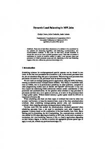
The key class denotes the topic of the publication; symbol represents the symbol of the stock and carries a string value of YHOO. The stock’s open, high, low, close, and volume values are numeric and hence unquoted. Subscribers issue subscriptions to specify the type of publications they want to receive. Depending on the implementation, subscription filters can be based on attributes (which this thesis focuses on) or paths by the use of XML [2, 27, 28]. Attribute-based predicates consist of an operator-value pair to specify the filtering conditions on each attribute. Some examples of operators used for string-type attributes include equal, prefix, suffix, and contains comparators, denoted as eq, str-prefix, str-suffix, and str-contains, respectively. For attributes containing numeric values, one can use the =, >, =, and ,300000] The space of interest defined by these filtering conditions is called subscription space. A broker’s covering subscription set (CSS) refers to the set of most general subscriptions whose subscription space is not covered by any other subscription in the broker. For example, if a broker has the following set of subscriptions: [class,eq,’STOCK’] [class,eq,’STOCK’],[symbol,eq,’YHOO’] [class,eq,’STOCK’],[volume,>,1000] [class,eq,’SPORTS’] [class,eq,’SPORTS’],[type,eq,’RACING’]

then its CSS is composed of just: [class,eq,’STOCK’] [class,eq,’SPORTS’]


8

Figure 2.1: Example of the poset data structure.

For more efficient retrieval of a broker’s CSS, the partially-ordered set (poset) [35] is used to maintain subscription relationships. The poset resembles a graph-like structure where each unique subscription is represented as a node in the graph. Nodes can have parent and children nodes where parent nodes have subscription space that is superset of its children nodes, while subscriptions with intersecting or empty relationships will appear as siblings. Hence, it is possible for a subscription to have more than one parent and children node in the poset. Figure 2.1 shows the poset for the five subscriptions given in the above example. As shown, the CSS is readily available as the immediate children nodes under the imaginary root node. Subscribers issue unsubscription messages whenever they disconnect from the system. Unsubscription messages do not contain any predicates, but an identifier that correlates to the subscription to be removed from the system. In some content-based publish/subscribe systems, such as SIENA [9], REBECA [24], and PADRES [19], advertisements are sent by publishers prior to sending the first publication message. For example, a publisher of the publication previously outlined would have an advertisement such as this:

[class,eq,’STOCK’],[symbol,eq,’YHOO’],[open,isPresent,0],[high,isPresent,0], [low,isPresent,0],[close,isPresent,0],[volume,isPresent,0], [date,isPresent,’00-00-00’]


9

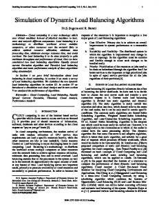
Figure 2.2: Example of content-based publish/subscribe routing.

Sometimes, it may not be always possible to know the exact range of an attribute’s value before publishing. Hence, the isPresent operator is used to denote that the attribute merely exists with a string or numeric type. Advertisements are flooded throughout the network so that subscriptions do not have to be flooded but instead travel in the reverse path of matching advertisements. In publish/subscribe systems without advertisements, subscriptions have to be flooded to guarantee no false-negatives in event delivery. Since publishers are assumed to be less dynamic and mobile than subscribers, the cost of flooding advertisements is far less than flooding subscriptions. This assumption holds true in real-world scenarios. For example, newspaper agencies rarely change, but the number of news readers subscribing and unsubscribing from a newspaper is comparatively much higher. Unadvertisement messages are used by the publisher whenever it disconnects from the system.

2.1.3

Content-based Publish/Subscribe Routing

Figure 2.2 demonstrates an example of how advertisements, subscriptions, and publications are routed. In the first step, the publisher (represented by a triangle) advertises a>1 to broker


10

B1. As shown by the arrows labeled with 1, the advertisement is flooded to all brokers in the network. Subscribers never receive advertisements because advertisements are control messages and subscribers should only receive publication messages that match its subscription filter. In step 2, subscriber sub1 issues its subscription a>5 to broker B4. Since sub1 ’s subscription’s space is common with the publisher’s advertisement space, sub1 ’s subscription is forwarded along the reverse path of the advertisement, as shown by the arrows labeled with 2. Notice that the publisher does not receive the subscription because subscriptions are control traffic within the publish/subscribe system and publishers never receive messages. In step 3, subscriber sub2 issues its subscription a>9 to broker B3. Similar to sub1 ’s subscription, sub2 ’s subscription travels in the reverse path of the publisher’s advertisement since it matches with a subset of the advertisement space. However, once the subscription reaches to broker B2, the subscription is purposely not forwarded to broker B1 because sub2 ’s subscription is covered by sub1 ’s. In other words, since B2 is already receiving publication messages that matches sub2 ’s subscription space due to sub1 ’s subscription, it is not necessary to forward sub2 ’s subscription to B1. As illustrated in the figure, publications sent by the publisher in step 4 will get delivered to both subscribers according to the brokers’ publication routing tables shown beside each broker (with the left and right columns representing the next-hop and subscription filter, respectively). When subscriber sub1 unsubscribes from broker B4 in the future, the unsubscription will traverse along the same path as sub1 ’s original subscription up to broker B1. When the unsubscription reaches broker B2, B2 should forward sub2 ’s subscription to B1 before sub1 ’s unsubscription to avoid interrupting sub2 ’s event delivery.

Subscription-covering reduces network overhead, broker processing load, and routing table size. Advertisement routing can also be optimized using the subscription covering idea where covered advertisements do not need to be forwarded. Other routing optimization such as subscription merging [24] and rendezvous nodes [29] may be employed to make the publish/subscribe system more scalable. However, hotspots can still arise because there is no load balancing mechanism.


2.1.4

11

Load in Publish/Subscribe

Load in a publish/subscribe system are introduced by publishers and subscribers that share the same information space. Publishers impose load by publishing messages into the system. However, without subscribers, the system stays idle because all publication messages are dropped at the publisher’s immediate broker. The same applies in the reverse case. If there are only subscribers, the system will never get loaded because no publications ever need to be matched and forwarded. Therefore, publishers and subscribers go hand-in-hand to impose load in a publish/subscribe system.

2.2

Load Balancing

Load balancing has been a widely explored research topic for the past two decades since the introduction of parallel computing. New load balancing techniques were invented as new technologies emerged to suit its needs, such as distributed systems, and the Internet. The following two subsections will examine previous works in load balancing and terminologies used for classifying load distribution algorithms.

2.2.1

Load Balancing in Different Software Layers

Load balancing solutions can be found in different software layers today, as shown in Figure 2.3. Starting from the bottom of the figure, load balancing at the network layer can be found in Internet routers and the Domain Name Service (DNS) [7, 8, 13]. For example, the DNS can perform load sharing by returning the IP address of the web server that is least loaded. Other distribution algorithms, such as random or round-robin are applicable as well. However, the effectiveness of DNS load sharing is hindered by the client’s caching mechanism that stores the name-to-address mapping. With the advent of personal computers, numerous load balancing solutions started appearing in the operating system layer that focused on distributing load onto a cluster of networked computers. Operating system solutions can be further classified as user-level or kernel-level. Examples of user-level load balancing solutions include Remote Unix [21], Emerald [17], Con-


12

Figure 2.3: Load balancing implementations at various software layers.

dor [22], and Utopia [41]. Examples of kernel-level solutions include Solaris MC [33] and OSF/1 AD TNC [40]. User-level implementations benefit from loose-coupling with the kernel. Therefore they can run on different versions and types of operating systems without requiring any modifications. However, they cannot perform full load balancing because some data structures may be hidden within the kernel that are not accessible from the user-level. Kernel-level implementations, on the other hand, are more efficient and effective because the overhead to user-space is eliminated, and all information about the kernel is readily available. However, they are less flexible compared to the user-level implementations because every new kernel version requires a complete reimplementation of the load balancing module. As distributed applications emerged, load balancing began appearing in the middleware layer to better suit to the application’s needs and yet provide load balancing services transparently. Research in load balancing at the middleware layer centre mostly around CORBA, which work at the object-oriented abstraction level. Similar to the classification of load balancing solutions with user and kernel-levels at the operating system layer, some middleware implementations operate outside of CORBA such as [1, 4, 16], while some operate within such as [20]. Because


13

the middleware layer sits on top of the operating system layer as shown in the Figure 2.3, middleware load balancing solutions can use load balancing tools offered at the operating system layer, such as process migration. Sometimes, load balancing facilities provided at the lower levels can be too general to be applied to an application’s load balancing requirements. This calls for the need to implement an application-specific load balancing solution. Such a solution can use the load balancing facilities in the middleware or operating system layer. An advantage of application-level load balancing is that it is effective on the application itself. However, a main disadvantage of this approach is that load balancing is no longer transparent to the application programmer [5, 26], and it may require full reimplementation whenever the application is updated. Because all existing approaches are too general to estimate the load of a subscription and account for subscription spaces, an explicit load balancing solution is needed to distribute load effectively in a heterogeneous content-based publish/subscribe system.

2.2.2

Classification of Load Distribution Algorithms

All load distribution algorithms are classified under a loosely unified set of terms, of which the original derivations came from Casavant et al. [10] and Shivaratri et al. [34]. All terminologies use the term processes to refer to resource consumers and processors as the resources. First, the terms load balancing and load sharing do not have the same meaning [34]. Load balancing takes on a best-effort approach to distribute load evenly onto every processor in the system at any point in time. On the other hand, load sharing is a subset of load balancing where load is distributed by initiating processes at idle processors. From the last definition, load sharing is non-preemptive, that is, processes never migrate once they are started. The use of the terms load sharing and load balancing will have these distinctive meanings from this point onwards. According to Casavant [10], load distribution algorithms can be classified under the hierarchy shown in Figure 2.4. First, an algorithm can be local or global. Local load distribution algorithms deal with scheduling processes on a single processor, whereas global deals with two or more processors. All load balancing solutions mentioned previously, as well as the proposed load balancing algorithm in this thesis belong to the global category. On the next level down,


14

Figure 2.4: Casavant’s classification of load distribution strategies.

a load distribution algorithm can be static or dynamic. A static algorithm makes load sharing decisions only when initiating a task/process. Once the process is assigned to a processor, it stays there until completion. A dynamic algorithm is much more flexible in that load balancing can trigger anytime when necessary, but requires handling process migrations that may be complicated. An adaptive load balancing algorithm takes the extra step of modifying the scheduling policy itself to account for system-state stimuli. On the next level below the dynamic category, an algorithm can be centralized or distributed. Centralized means that all load balancing decisions are made at one processor, while distributed means that the same decisions are made in a distributed fashion. Centralized approaches are ignored in this work because they are not scalable [18, 23, 34] and they introduce a single-point-of-failure in the system. Other terminologies shown in Figure 2.4 are not referred extensively in this thesis and hence not defined here.


2.3

15

Related Work

Although distributed content-based publish/subscribe systems have been widely studied over the past few years, the topic of load distribution is rarely addressed. Hence, the proposed solution in this thesis is the first dynamic load balancing algorithm for content-based publish/subscribe systems to date. Terpstra et al. [36] proposed a peer-to-peer content-based publish/subscribe system that is based on a distributed hash table (DHT) routing backbone. However, their load distribution technique is very briefly mentioned with no supportive experimental data. Load distribution in Terpstra’s system is accomplished by having a different publication dissemination tree at every broker/peer. However, for this to work effectively, publishers must be distributed evenly across all peers in the system. This problem becomes even more difficult when publishers have different publication rates that vary in time. Unfortunately, none of these issues are addressed. Meghdoot [15] is a peer-to-peer distributed content-based publish/subscribe system based on DHT for efficient assignment of subscription space onto peers. Clients in Meghdoot form the broker overlay network, and they can be a publisher, subscriber, or both. Its load distribution algorithm relies on two load indices to make load sharing decisions: event propagation, which is based on the number of events delivered; and subscription management, which is the number of subscriptions managed in a zone. Based on these load indices, a new joining peer either replicates the highest loaded peer’s zone, or split the peer’s zone in half so that each peer ends up with half of the number of subscriptions in the original zone. The latter action assumes that all peers are homogeneous, meaning they have equal resources capacities. Since load balancing is only triggered whenever a new node joins the system, Meghdoot’s load distribution algorithm is considered to operate statically. This static nature means that it cannot redistribute load from overloaded brokers if there are no new joining peers. Chen et al. [11] proposed a dynamic overlay reconstruction algorithm that reduces end-toend delivery delay and also performs some load distribution in the process. Several properties of their load distribution algorithm can be devised from their home broker1 selection methodology. 1

Equivalent to the term immediate broker used in this thesis


16

First, their load distribution is based on one load index, which is the CPU load. Second, load balancing is triggered only when a client finds another broker that is closer than its home broker, which only happens if nodes are mobile. This means that the load distribution algorithm will never get invoked in a static environment. Third, overloaded brokers cannot trigger load balancing themselves, but have to rely on the clients’ detection algorithm. This may prevent an isolated cluster of brokers from relieving their overload condition if a hotspot arises and all clients are closest to this cluster of brokers in the entire federation. As a result, all overloaded brokers in that cluster will eventually crash. Fourth, subscriber migrations may overload a non-overloaded broker if the load requirements of the migrated subscription exceed the loadaccepting broker’s processing capacity. By contrast to these related works, the load balancing solution proposed in this thesis is applied to publish/subscribe systems having dedicated servers for brokers, and eliminates all of the limitations from the previous approaches. First, the solution presented here accounts for heterogeneous brokers and subscribers. Experiments show that the load balancing algorithm can load balance with brokers up to 10 times the difference in resource capacities, and handle subscribers with publication traffic that vary from zero to all publications published into the system. Second, load balancing can happen dynamically, such as when a broker is overloaded, and not restricted to new client joins. Third, all load balancing actions will not overload the load-accepting broker to maintain reliability and availability of the system. This is ensured by having a load estimation algorithm that predicts the load of the load-accepting broker before the offload occurs. Load estimation does not exist in any of the previous works. Fourth, the proposed solution load balances on three load indices, versus two as in Meghdoot, and one as in [11]. Matching delay is almost the equivalent to Meghdoot’s subscription management load index, but matching delay is a better index because it accounts for brokers with different processing power as well. Finally, the proposed solution uses a best-effort approach to balance all three load indices simultaneously. In contrast to Meghdoot, node splitting evens out the subscription management of each peer, but not the event propagation as subscriptions are heterogeneous. [11] does not attempt to distribute load evenly because its primary concern is reducing delivery delays and not load balancing.

Chapter 3

Load Balancing Framework 3.1

Overview of Load Balancing Components

Figure 3.1: Components of the load balancer.

The components that make up the load balancing solution are shown in Figure 3.1. It consists of the detector, mediator, load estimation tools, and offload algorithms that determine which subscribers to offload. The detector detects when an overload or load imbalance occurs. The mediator establishes a load balancing session between the two entities, namely offloading broker (broker with the higher load doing the offloading) and the load-accepting broker (broker 17

Chapter 3. Load Balancing Framework

18

accepting load from the offloading broker). An offload algorithm is invoked on the offloading broker to determine the set of subscribers to delegate to the load-accepting broker based on estimating how much load is reduced and gained on each broker. Finally, the mediator is invoked to coordinate the migration of subscribers and ends the load balancing session. The following sections will describe the load balancing framework and the operations of each component in greater detail.

3.2

Underlying Publish/Subscribe Architecture

Figure 3.2: Publish/subscribe architecture with PEER.

In standard publish/subscribe systems, all brokers are classified equally, and clients connect to the closest broker in the network. With Padres Efficient Event Routing (PEER) shown in Figure 3.2, brokers are classified into two types, and clients can only connect to either one type of these brokers. Brokers with more than one neighboring broker are referred to as cluster-head brokers, while brokers with only one neighbor are referred to as edge-brokers. A cluster-head broker with its connected set of edge-brokers form a cluster. Brokers within a cluster are assumed to be closer to each other in network proximity than brokers in other


19

clusters. Likewise, brokers in neighboring clusters are closer to each other in network proximity than brokers more than one cluster-hop away. Publishers are serviced by cluster-head brokers, while subscribers are serviced by edge-brokers. PEER is applicable only if there are three or more brokers in the federation. Thus, with one or two brokers in the system, brokers are not given any classification, so publishers and subscribers can be serviced by any broker. However, when the third broker connects to a federation with two brokers, the broker accepting the connect request detects that it has more than one neighbor, and changes its role to a cluster-head and tells its neighbors to take on the role of edge-brokers. In this conversion process, the cluster-head has to migrate away all subscribers to the edge-brokers randomly, and the edge-brokers have to migrate away all publishers to the cluster-head. This conversion process is repeated whenever a new broker connects to an edge-broker. Control subscriptions and publishing agents vital to the operation of brokers are exempted from the migration process in PEER and load balancing. This PEER-based design offers three key advantages: higher efficiency in publication dissemination, reduced load balancing overhead, and increased subscriber locality. First, clusterheads can forward publication messages to all matching clusters almost simultaneously because cluster-heads have negligible processing delays since they do not service any subscribers. Because cluster-heads in PEER have very light loads, they rarely become overloaded and thus can operate reliably without load balancing. Edge-brokers, on the other hand, need to be load balanced since they bear the majority of the matching and forwarding load, and they are also susceptible to overload because of the likelihood of uneven distribution of subscriber population and interests. Second, PEER’s organization of brokers into clusters allows for two levels of load balancing: local-level (referred to as local load balancing) where edge-brokers within the same cluster load balance with each other; and global-level (referred to as global load balancing) where edge-brokers from two different clusters load balance with each other. In local load balancing, edge-brokers only need to exchange load information with edge-brokers in the same cluster. In global load balancing, neighboring clusters can exchange aggregated load information about their own edge-brokers. Compared to global broadcast, message overhead is tremendously reduced. Third, local load balancing preserves subscriber locality by migrating subscribers only


20

among edge-brokers within a cluster. Using this scheme, subscribers are slowly diffused, clusterby-cluster, until the load difference between the clusters are below the global load balancing threshold. This is specifically tailored to adapt to real-life usage scenarios where publishers and subscribers with similar interests usually reside in the same geographical location. For example, residents in Toronto are more interested in local Toronto news than any other cities in the world. Not surprisingly, local news about Toronto are also published in Toronto. It is very rarely that residents in Vancouver are more interested in news about Toronto than Vancouver, and news about Toronto are almost never published from Vancouver. Therefore, it is beneficial to keep the subscriber as close as possible to its original cluster to reduce bandwidth consumption in the publish/subscribe backbone. To give clients more flexibility to the PEER structure, publishers and subscribers are free to connect to any broker as its first step. If a publisher connects to an edge-broker, the broker will redirect the publisher to its immediate cluster-head broker. If a subscriber connects to a clusterhead broker, the broker will redirect the subscriber to a randomly chosen edge-broker that is not overloaded (more on how to detect this later in the Section 3.3.1). Though, a more elegant solution exists where the cluster-head can smartly choose the least loaded broker to forward the subscriber. However, it is not always simple to choose which broker is least loaded, considering that there are three load indices to consider, and a subscription may or may not greatly affect the input utilization ratio of a broker without knowing the broker’s covering subscription set. Since the proposed load balancing solution operates dynamically, the subscriber can connect to any edge-broker first, and let the load balancer handle any uneven load distribution afterwards. Experiments show that the proposed load balancing solution can handle the case where all subscribers connect to one edge-broker on network startup. Therefore, a dynamic algorithm covers the need for any complex static solutions.

3.3

Load Detection Framework

Detection allows a broker to trigger load balancing whenever it is overloaded or has a large load difference with another broker in the system. In order for brokers to know which other


21

brokers are available for load balancing, a scalable messaging framework with minimal overhead is needed.

3.3.1

Protocol for Exchanging Load Information

Padres Information Exchange (PIE) is a distributed hierarchical protocol for exchanging load information between brokers using the underlying publish/subscribe protocol. PIE is developed to operate in a fully distributed manner so that it inherits and preserves the distributed properties of the existing publish/subscribe system, including scalability and no single-point-of-failure. Its hierarchical operation follows the organizational structure offered by PEER to achieve higher efficiency and reduced overhead. Because it operates on the existing publish/subscribe protocol for routing, PIE is simple and readily applicable to other publish/subscribe systems as well. Brokers publish PIE messages intermittently to let other brokers in the federation know of its existence and its availability for load balancing. Through PIE, brokers who find themselves more loaded compared to other brokers can initiate load balancing with the least loaded broker available. PIE, as well as other load balancing control messages described in later sections, has a higher routing priority than normal publish/subscribe traffic. This allows input overloaded brokers to receive PIE messages immediately without the added input queuing delay, and output overloaded brokers to send load balancing requests immediately. PIE publication messages contain the following pieces of information stored as attribute key-value pairs: BrokerID - the unique identification string of the broker ClusterID - the unique identification string of the cluster to which the broker belongs. This parameter differentiates PIE messages routed in different clusters Status represents the load balancing state of the broker or cluster in the case of local or global load balancing, respectively. It can be one of the following states: OK - ready to invoke or accept a load balancing request BUSY - currently load balancing with another broker/cluster and cannot initiate/accept a new load balancing session until the current one is finished


22

N/A - not available for load balancing. For edge-brokers, it means that it is overloaded. For a cluster, it means that it has at least one overloaded edge-broker. A broker/cluster with this status cannot accept load balancing requests, but it can initiate load balancing to do offloading. STABILIZING - in the final stage of load balancing where it just finished accepting or offloading subscribers and is waiting for load to stabilize State transitions for local and global load balancing are shown in Figures 3.3a and 3.3b, respectively. Balanced Set - set of brokers with which this broker is balanced. This is used for terminating global load balancing sessions Matching Delay (dm ) - load index defining the average matching delay of the broker Input Utilization Ratio (Ir ) - input load index defined by the formula: Ir =

ir mr

(3.1)

where ir is the incoming publication rate to the broker’s input queue, and mr is the maximum matching rate of the broker’s matching engine. mr is defined by: mr =

1 dm

(3.2)

A Ir greater than 1.0 means that the input resource is overloaded because the incoming message rate is higher than the matching rate, which may lead to an unbounded input queue size. Output Utilization Ratio (Or ) - output load index defined by the formula: Or =

ou ot

(3.3)

where ou is the output bandwidth used, and ot is the broker’s total output bandwidth. A Or greater than 1.0 means that the output resource is overloaded because there is insufficient bandwidth to cope with the message rate produced by the matching engine, which can lead to an unbounded output queue size.


23

By looking at the fields in the PIE message, it shows that the load balancing solution balances three resource bottlenecks of a broker, namely input utilization ratio, output utilization ratio, and matching delay. Alternatively, it is also possible for the load balancer to use input queuing delay and output queuing delay in place of their utilization ratio counter-parts. However, using queuing delay measurements do not accurately indicate the load of a broker at the instant the value is measured because it is obtained after the message gets dequeued. So the measurement is lagging by the delay measured. For the messages that follow, they may experience much higher or lower delays if the enqueue rate increased or decreased after the sampled message. On the other hand, calculating utilization ratio requires sampling the message rate at the time when messages get enqueued. Therefore, by using utilization ratios for detection and load estimation, the load balancing convergence time is reduced because triggering can happen earlier, and load estimation is more accurate. PIE messages are control messages that add overhead to the publish/subscribe routing infrastructure. Frequently publishing PIE messages can keep load information up-to-date at neighboring brokers, but add unnecessary overhead if the messages contain unchanged load information. To make PIE as efficient as possible, the following parameters are used to coordinate its publication activities: Utilization Ratio Threshold - Do not publish a PIE message if the current utilization ratio load indices do not differ from the previous published corresponding values by more than this threshold Delay Threshold - Do not publish a PIE message if the current delay load indices do not differ from the previous published corresponding values by more than this percentage difference threshold Generation period - By default, PIE messages are generated periodically defined by this parameter When a PIE message is generated, it has to meet certain criteria in order to get published. First, at least one of the three load indices must past a threshold defined above. Load indices


(a) A broker in local load balancing.

24

(b) A cluster in global load balancing.

Figure 3.3: State transition diagrams.

that do not past the threshold value are considered redundant information and hence are not published. Second, the current load balancing status must be OK, or the current status has changed compared to the previous one. Brokers with a status of OK are available for load balancing and hence should publish PIE messages. Brokers with a status changed from BUSY or N/A to OK should publish a PIE message to let its neighbors know that it is now available for load balancing again. However, brokers whose status remains unchanged from N/A, BUSY, or STABILIZING do not need to publish another PIE message because subsequent PIE messages have no effect on neighboring brokers’ load balancing decisions. A diagram showing the transition conditions between the local and global load balancing states are shown in Figures 3.3a and 3.3b, respectively.

Upon receiving a PIE message from a neighboring broker, data from the message is stored into a data structure for future reference. This data is stored for a duration of 3× the generation period, starting when the message is received. This feature prevents too much staleness in the data, and enables automatic removal of entries for brokers that have left the federation. However, this will require brokers to publish PIE messages at every other generation period in order to preserve its PIE entry at neighboring brokers.

Chapter 3. Load Balancing Framework 3.3.1.1

25

Load Exchange Protocol for Local Load Balancing - Local PIE

Since edge-brokers can initiate local load balancing with any brokers they learn through PIE, enforcing local load balancing only requires limiting the dissemination of local PIE messages within the publisher’s cluster. This is easily achievable through publish/subscribe by having edge-brokers subscribe to PIE messages with the clusterID attribute set to the cluster to which they belong. For example, an edge-broker in cluster C1 will issue the following subscription to subscribe to its own cluster’s local PIE messages: [class,eq,’LOCAL_PIE’],[clusterID,eq,’C1’] Publishers follow a similar rule where they have to publish local PIE messages with the clusterID attribute set to its own cluster. For example, edge-brokers in cluster C1 will have to publish local PIE messages with the clusterID set to C1 : [class,’LOCAL_PIE’],[clusterID,’C1’],... By using the underlying publish/subscribe infrastructure, no additional routing logic needs to be implemented to limit PIE messages from disseminating to neighboring clusters. Additionally, routing PIE messages between clusters can be easily controlled by adding or removing subscriptions dynamically. Compared to broadcasting, this method is more flexible and reduces network overhead. 3.3.1.2

Load Exchange Protocol for Global Load Balancing - Global PIE

Global PIE messages contain summarized load information about a cluster. This load information consists of the input utilization ratio, matching delay, and output utilization ratio, taken from the average of all edge-brokers in the cluster. Averaging the load indices will give a rough indication of the cluster’s load after load balancing has converged. In a heterogeneous scenario, this estimation scheme may not yield a prediction as accurate as if all brokers in the cluster have equal resource capacities. With a dynamic load balancing algorithm active at all times, load differences between brokers are automatically reduced. Therefore, estimation error from the average function is also reduced. For global PIE, estimations do not have to be very accurate,


26

and given the simplicity of the average function, the tradeoff between accuracy and simplicity is acceptable. As mentioned previously in the section on PEER, a cluster can only invoke global load balancing with its neighboring clusters to promote locality for subscribers. This scheme is supported by limiting the propagation of global PIE messages to one cluster-hop away. Consequently, cluster-heads only know about its immediate neighbors. An exception applies if a cluster is N/A, which allows it to forward incoming global PIE messages to all of its immediate cluster-head neighbors. This prevents unavailable clusters from acting as ”barriers” to normal clusters that can do global load balancing.

3.3.2

Triggering Load Balancing Based on Detection Results

Detection allows a broker/cluster to monitor its current resource usage and also compare it with neighboring brokers/clusters so that it can invoke load balancing if necessary. To make load balancing invocations more stable and accurate, the detector operates on load indices that are smoothed out by the formula: yn = α · x + (1 − α) · yn−1

(3.4)

where yn is the load index used for detection purposes, x is the current load index value, yn−1 is the load index used in the previous detection run, and α is a configurable variable. A higher α value will give a more accurate result to the present value, but may exhibit more fluctuations if there are large peaks in the load. A lower α will give a more smoothed result, but may slow down the reaction time of the detector. Detection runs periodically at a broker/cluster only if it has a status of OK, meaning it is available for load balancing; N/A, meaning it is overloaded; and STABILIZING, meaning it is waiting for load to stabilize after load is exchanged. It does not run when the broker/cluster has a status of BUSY, meaning it is currently in a load balancing session. In between detection runs, the detector sleeps for a random amount of time governed by the minimum and maximum detection period parameters. The detector is awakened by incoming PIE messages with an OK status to give faster load balancing response times. The detection schemes for local and global load balancing differs slightly, therefore they will be explained separately below.


27

Figure 3.4: Illustration of a broker’s response to overload.

3.3.2.1

Triggering Local Load Balancing Based on Local Detection Results

The local detection algorithm is composed of two steps. The first step identifies whether the broker itself is overloaded by examining four utilization ratios, namely: • Input utilization ratio • Output utilization ratio • CPU utilization ratio • Memory utilization ratio Identifying an overloaded broker is critical because a broker in its overloaded state (i.e., when the utilization ratio is greater than 1) can lead to high queuing delays, instability, and unavailability. Therefore, as shown in Figure 3.4, a lower overload threshold parameter is introduced that marks the broker as N/A if any one of its resources past this mark so that the broker is prevented from accepting more load. This parameter is set to 0.9 by default. If a utilization ratio exceeds the higher overload threshold (shown to be 0.95 in Figure 3.4), then load balancing is invoked immediately. In between the two thresholds is an inert period where the broker neither accepts nor invokes load balancing. If a utilization ratio exceeds the upper overload threshold, then the detector will tell the trigger which resource is overloaded so that the trigger will immediately invoke the appropriate


28

load balancing action with the most suitable neighboring broker found through PIE. If the input utilization ratio is overloaded, then the trigger will pass to the mediator a list of broker ids of brokers found through PIE not having a N/A status, sorted in ascending order of input utilization ratio. These broker ids will be associated with a load balancing action of type input for load balancing the input utilization ratio. This way, the mediator will try to initiate input load balancing with the broker that is least input utilized first. If the output utilization ratio is overloaded, then a list of broker ids all associated with the load balancing action output sorted by ascending output utilization ratio is passed to the mediator for output load balancing. If the CPU or memory usage is overloaded, then a list of broker ids all associated with the action match sorted by ascending matching delay is passed to the mediator for match load balancing. If more than one resource is overloaded, then first load balance the resource with the highest utilization ratio. An exception arises if the input utilization ratio is also overloaded. In this case, regardless of the other utilization ratios, perform input load balancing first because this action will reduce the matching delay and all other utilization ratios as well. For more details on the input, output, and match offload algorithms, please refer to Section 4.2. If the first step of the detection algorithm cannot find any overloaded resource, then the second step is invoked to balance the input, match, or output load indices with neighboring brokers found through PIE. Load balancing is only invoked by the broker having the higher load index and the difference between the two broker’s load indices must exceed a threshold in order for any triggering to occur. For input and output utilization ratios, the difference between the two brokers’ values must exceed the local ratio threshold parameter, which is set to 0.1 by default. For matching delay, the percentage difference between the two broker’s delay values must exceed the local delay threshold parameter, which is also set to 0.1 by default. The formula to calculate the percentage difference of two delay values is: d%Dif f =

d1 − d2 Nf

(3.5)

where d1 and d2 are the two delay values used in the comparison. Usually, in percentage difference calculations, the denominator is either the value of d1 or d2 . However, this introduces two problems. First, extremely low delay values may yield a high percentage difference although


29

the magnitude of the difference is negligible. For example, it is impractical to load balance on a matching delay percentage difference of 50% if the two values are 0.000002s and 0.000001s. Second, extremely high delay values may only load balance when the magnitude of the difference is large. For example, if the delay threshold is 10%, then a broker with matching delay of 10s will only invoke load balancing with another broker having a matching delay of 9s or less. This 1s matching delay difference is far too large. Hence, a normalization factor, Nf , is used at the denominator instead. Its value is set to 0.1 by default, which normalizes percentage differences to 0.1s. Logically, the neighboring broker having the highest load difference should be chosen for load balancing on the particular load index of interest. If that neighbor is not available, then the next neighbor having a load difference that is second highest is chosen. From this pattern, a brokeraction list of {broker, load balancing action} can be generated that is sorted in descending order of highest load index difference. The list is then passed to the Mediator (see Figure 3.1) to physically establish a load balancing session with an available broker. So far, the local detection scheme described seems to work fine. If any resource is overloaded, it will mark the broker as N/A and invoke the appropriate load balancing algorithm to relief the overload. If nothing is overloaded, it will mark the broker as OK and can possibly invoke load balancing to distribute load evenly among neighboring brokers. However, a stability issue arises if the detector triggers another load balancing session immediately after a previous one. If the broker was an offloading broker in the previous load balancing session, its load indices may not be given enough time to drop to a stabilized level. Consequently, the detector may invoke load balancing on a load index that have not stabilized yet, which can make the broker’s final load drop far below what is expected. Likewise, if the broker was a load-accepting broker in the previous load balancing session, its load indices may not have risen to a stable point yet. Thus it will continue to accept more load from other brokers and end up with more load than expected. Together with both cases, load will constantly swing back and forth between brokers, leading to never ending instability. To prevent this problem from happening, a broker inherits a status of STABILIZING after it finishes a load balancing session. It regains a status of OK only if no overload occurs and it must satisfy two constraints. These constraints are applied


30

between the first and second step of the detection algorithm described above to allow local load balancing to occur while stabilizing only if a resource surpasses the upper overload threshold. The first constraint prevents the second step of the detection algorithm from running for a certain number of detection cycles as specified by the configuration parameter stable duration. However, a fixed amount delay may give too much stabilization time for a load balancing session that exchanged very little load, or too less for a session that exchanged a large amount. Hence, a second constraint is introduced to allow for more flexible stabilization time. This second constraint prevents the detection algorithm from running if any one of the three load indices have not stabilized to within a percentage for a given period of time. The parameter that controls this is called stable percentage, which means a percentage change less than this parameter over a 60s (hard-coded) time interval is considered to have stabilized. Figure 3.5 summarizes the entire local detection algorithm.

3.3.2.2

Triggering Global Load Balancing Based on Global Detection Results

As shown in Figure 3.3b, a cluster in global load balancing uses the states: BUSY, N/A, and OK, to indicate its current load balancing status. A cluster has a BUSY status if it is currently load balancing with another cluster. N/A is assigned to signify that the cluster is not available for load balancing if any one of its edge-brokers are overloaded. This allows the overloaded brokers to offload subscribers to brokers within the same cluster first to promote locality. An OK status denotes that the cluster is not currently participating in any global load balancing and none of its edge-brokers are overloaded. Consequently, a cluster can accept global load balancing requests only if its status is OK. If the cluster is identified to be BUSY, then detection is aborted to avoid initiating another load balancing session. Otherwise, neighboring clusters learned through global PIE are selected for load balancing if the difference of a load index between the two clusters exceed a triggering threshold. Load index differences are calculated using the same formulas as in the local detection algorithm described in the previous section. For those clusters with a load index surpassing the threshold, they are put into a list sorted by descending highest load difference. The end result will be a sorted list of clusters to try to initiate global load balancing. This list then gets passed


Figure 3.5: Flowchart of local detection algorithm.

31


32

to the global mediator to establish a global load balancing session. Details on the operations of the global mediator are given in Section 3.4.3. For greater flexibility, threshold values for ratio and delay measurements used in the global detection algorithm are defined separately from the local detection algorithm. Those used in the global detection algorithm are called global ratio threshold and global delay threshold. In order for the global detection algorithm to work effectively with the local version, global thresholds should be set higher or equal to the local equivalents. If this condition is not met, then there will be a contradictory condition where at the local-level, edge-brokers appear balanced, but at the global-level, they are not. Global load balancing can also be initiated anytime when an overloaded edge-broker cannot find any edge-brokers in its own cluster to load balance, as shown in Figure 3.5. In this case, the overloaded edge-broker will send a global load balancing request publication message to its cluster-head telling it to initiate global load balancing. If the cluster is currently not BUSY, then the cluster-head will run the global detection algorithm to initiate a global load balancing session with a neighboring cluster. If the cluster is currently BUSY, then it means that the overloaded edge-broker cannot load balance with any edge-brokers in both clusters. Hence, the cluster with the overloaded edge-broker will cease the current global load balancing session and initiate a new one with another cluster after receiving N number of global load balancing requests. The parameter N is called global load balancing request threshold.

3.3.2.3

Optimization to Reduce Load Balancing Response Time

Every broker has an equal opportunity to invoke load balancing with another less loaded broker, and brokers accept load balancing requests based on a first-come-first-serve basis. This is a fair protocol allowing each broker to have equal competition. However, sometimes it may be more preferable to allow more loaded brokers, especially overloaded ones, to have higher priority for requesting load balancing over lesser loaded brokers. This biasing offers two benefits. It can help to improve response time of the load balancing algorithm because this helps to spread isolated load to other brokers immediately before all brokers load balance on a finer level. Reliability and availability is also improved because overloaded brokers spend less time overloaded and


33

have lower peak utilizations by being able to invoke load balancing sessions more readily. Implementation of this prioritizing scheme adds no complexity to the existing detection algorithm. Instead of brokers being able to trigger load balancing sessions whenever they wish, they must first check to see if any brokers have a status of N/A in the PIE messages received. If one exists, and the broker running this detection has an OK status, then do not invoke any load balancing sessions. Brokers that are overloaded (i.e., N/A) are exempted from this check so that they are prioritized ahead of OK brokers. Once the N/A brokers have initiated their load balancing sessions, their status will appear as BUSY in their PIE messages. At this point, any remaining OK brokers that are not load balancing with the overloaded brokers are free to invoke load balancing as needed. In the grand picture, this optimization allows overloaded brokers to invoke load balancing before normally loaded brokers. It is applied to both local and global detection/triggering schemes. Its implementation on both local and global levels are the same, because both triggering schemes use PIE information, and both edge-brokers and cluster-heads use almost the same load balancing states.

3.4

Load Balancing Mediation Protocols with Brokers and Subscribers

All load balancing activities are coordinated by exchanging messages using the underlying publish/subscribe infrastructure for simplicity and efficiency. Specifically, request-reply and one-way protocols are implemented in publish/subscribe to coordinate broker and subscriber activities. The following paragraph will explain the request-reply implementation as it is a superset of the one-way protocol. Request-reply is used in setting up a load balancing session when an edge-broker, called B1, wants to do local load balancing with another broker, called B2. First, B1 needs to send a request to B2 asking if B2 is willing to load balance with it. After B2 receives this request, it sends a reply back to B1 indicating its acceptance or decline to the request. Both the request and the reply are publication messages. In order for this to work in publish/subscribe language,


34

both brokers B1 and B2 have to subscribe prior to sending the request/reply message. For example, broker B1 ’s subscription will specify the brokerID attribute to have a value equal to its own id to get request-reply messages sent for it: [class,eq,’LB_CONTROL’],[brokerID,eq,’B1’] Broker B2 ’s subscription also looks similar to the above subscription, except that the value of the brokerID attribute is set to B2 instead of B1. This methodology assumes that brokers have unique identifiers, and therefore, no two brokers will ever subscribe to the same message set. After setting up these subscriptions, broker B1 can send a request-reply message to broker B2 by creating a publication having the following required attributes: [class,’LB_CONTROL’],[brokerID,’B2’],... One of the key purposes of the load balancing algorithm is to allow overloaded brokers to transfer load to other less loaded brokers in the network. An overloaded broker may be input overloaded, where its input queue has a long line-up of messages waiting to be matched, or output overloaded where the output queues have a lot of messages waiting to be sent out. In either case, an overloaded broker will try to initiate a load balancing session with a less loaded broker to do offloading. First, the overloaded broker will send out a load balancing request message. If the requesting broker is output overloaded, then this message may take unnecessarily long time to get to the replying broker because of the high output queuing delay. Similarly, if the requesting broker is input overloaded, then the response from the replying broker will take a very long time because of the high input queuing delay. In both cases, the overloaded broker is not able to get immediate response from the less loaded broker, which results in slow response time of the load balancing algorithm, and further increasing the load of the overloaded broker, making it even more likely to crash. To avoid this problem, load balancing control messages must be given higher priority than normal publish/subscribe traffic. Messages that tell the subscribers to migrate, as well as the migrating subscribers’ subscriptions and unsubscriptions, have higher priority to promote faster response time of the algorithm and also reduce the likelihood of a crash from an overloaded broker.


3.4.1

35

Mediating Local Load Balancing

Once the local detection algorithm composes the broker-action list of candidate brokers for load balancing, the mediator of the requesting broker will send a load balancing request to the first broker in the list. When the replying broker receives this request, it is passed to its mediator to generate a reply. If that broker replies with a status of OK, then a load balancing session is started. Otherwise, the requesting broker’s mediator will send a request to the second broker in the list. This process repeats until an OK reply is received, or all brokers have rejected. If the latter case is true, and if the requesting broker is currently overloaded, then a global load balancing request publication message is sent to the cluster-head to initiate global load balancing, as previously shown in Figure 3.5. When the mediator of a replying broker gets a load balancing request, it first has to check its current load balancing status. If it is N/A, then it means that one of the load indices are overloaded and therefore should reject this request by sending back a reply with a N/A status. If it is BUSY, then it means that the broker is already doing load balancing with another broker, and should reply back with BUSY. Otherwise, if the status is OK, then it means nothing is overloaded, and it is not doing any load balancing. Consequently, the mediator will accept the load balancing request by replying with a status of OK and at the same time changes its current status to BUSY so that it does not engage in any other load balancing activities until the current one is done. The reply message also contains extra load information about the replying broker for the requesting broker to compute the set of subscribers to offload. This load information includes: • Covering subscription set • CPU utilization ratio • Input bandwidth usage • Input queue memory usage • Input publication rate • Matching delay slope


36

• Total memory • Total output bandwidth • Number of subscriptions • Output bandwidth used • Output queue memory usage When the requestor receives a reply with an OK status, it too changes its status to BUSY. The requestor can now trash the broker-action list because it found a partner to load balance with. Load information received in the reply message is then sent to the appropriate offload algorithm (one of input, output, or match) to determine the set of subscriptions to offload to balance the specific load index among the two brokers.

3.4.2

Mediating Subscriber Migration

Once the offloading algorithm is done with its computation, it returns back to the mediator a list of subscription identifiers of subscribers to offload. The mediator has to migrate the indicated subscriptions to the new broker in the most efficient and timely manner, and yet try to maintain 100% delivery ratio to the migrating subscribers. First, the mediator sends a control publication message to each subscriber in the offload list telling them to issue its subscription to the load-accepting broker. Subscribers issue a subscription to the load-accepting broker containing the ID of the load balancing session and the total number of migrating subscribers. These two pieces of information allow the load-accepting broker to know when it has received all migrating subscribers in the current load balancing session. For efficiency and best-effort guarantee of minimal delivery loss, the load-accepting broker waits for N × the migration timeout for all migrating subscribers to connect, where N is the total number of migrating subscribers. When all subscribers have connected to the load-accepting broker, or when the timeout occurs, the load-accepting broker sends a DONE control publication message back to the offloading broker to terminate the load balancing session. This message ensures that the publication path for all migrated subscribers have been setup to flow to the load-accepting broker. When the


37

offloading broker receives the DONE message, it tells the migrating subscribers to wait for all the messages currently in the offloading broker’s input queue to be matched and delivered from the output queues before sending a unsubscribe message to the offloading broker. A soft guarantee can be made by having the subscribers wait for the offloading broker’s current input queuing delay, plus the matching delay, plus the output queuing delay before unsubscribing. Once the migrating subscribers unsubscribe from the offloading broker, the migration process is complete.

3.4.3

Mediating Global Load Balancing

In local load balancing, edge-brokers themselves coordinate with each other to establish local load balancing sessions. On the cluster level, cluster-head brokers coordinate with each other to establish global load balancing sessions. The coordination protocol at the global-level is similar to that used at the local-level. First, the global mediator receives from the global detector a list of cluster-heads to contact to set up global load balancing. Cluster-head brokers receiving this message replies back with the current load balancing status of the cluster. On any reply other than OK, the requestor will try to contact the next cluster-head in the list until the list is exhausted. If the replying cluster-head has a status of OK, then it has to tell all edge-brokers in its own cluster to subscribe to the requesting cluster’s local PIE messages. Similarly, when the requesting cluster-head receives an OK reply for its request, it orders all edge-brokers in its own cluster to subscribe to the replying cluster’s local PIE messages. The point of subscribing to each other’s local PIE messages is to allow edge-brokers to learn about the existence and load indices of edge-brokers in the other cluster so that local load balancing can initiate between them. In the end, load is dispersed among edge-brokers in both clusters. Meanwhile, cluster-heads from both clusters continually monitor the balanced set field in local PIE messages exchanged between the edge-brokers to determine when to end the global load balancing session. Monitoring is made possible by having the cluster-heads subscribe to the other cluster’s local PIE messages as well. The balanced set lists all ids of brokers with whom a particular edge-broker is balanced with. When all edge-brokers publish local PIE messages with the balanced set containing all edge-brokers’ ids from both clusters, then it means that


38

local load balancing between the two clusters have converged to a steady state and global load balancing is done. When either cluster’s cluster-head decide to end the current global load balancing session, it has to send a DONE publication message to the other cluster-head. Upon sending or receiving a DONE message, the cluster-head tells its immediate edge-brokers to unsubscribe from the other cluster’s local PIE messages and remove them from their records to prevent further local load balancing between the two clusters. The cluster-heads themselves also unsubscribe from the other cluster’s local PIE messages because it no longer needs to monitor them.

Chapter 4

Load Balancing Algorithm 4.1

Load Estimation Algorithms

A dynamic load balancing algorithm requires knowledge about the individual brokers’ load information and resource capacities in order to select the least loaded broker to load balance with. Once a broker is selected, how many and which subscriptions are required to offload for balancing a particular load index between the two brokers? The following subsections will answer this question.

4.1.1

Estimating the Input and Output Load Requirements of Subscriptions

Padres Real-time Event-to-Subscription Spectrum (PRESS)1 is a space and time-efficient technique for estimating the bandwidth requirements and common publication set of two or more subscriptions based on current events. It uses bit vectors to record the matching pattern of subscriptions, hence the term event-to-subscription. It does not require the publish/subscribe system to use advertisements, nor does it assume that publications are in any sort of distribution. The operation of PRESS is best explained as part of the local load balancing algorithm after the mediation step where two brokers have agreed to load balance with each other. First, the offloading broker locally subscribes to the covering subscription set (CSS) of the load-accepting broker (as supplied in the OK reply message from the replying broker). Locally 1

Real-time refers to sampling using live incoming publications to the broker

39

Chapter 4. Load Balancing Algorithm

40

subscribe means that subscriptions are sent to the matching engine, but never get forwarded to neighboring brokers. This is sufficient because the offloading broker only wants to know which publications it currently sink are also received by the load-accepting broker. Next, all client subscriptions in the matching engine are allocated a bit vector of length N, where N represents the number of samples. Sampling starts immediately after getting the load-accepting broker’s OK reply message and ends after N publications are received or a timeout T is met, whichever comes first. Both N and T are configurable parameters referred to as PRESS samples and PRESS timeout, respectively. The algorithm starts at the right-most position of the bit vector for all subscriptions. A 1 is set if the subscription matched the incoming publication, 0 otherwise, before moving onto the next bit on the left. During the sampling period, the total incoming publication rate is measured. Tables 4.1a and 4.1b shows an example of the bit vectors with N = 6 for subscriptions at the offloading broker and load-accepting broker, respectively, given the following publication arrival order: 1. 2. 3. 4. 5. 6.

[class,’STOCK’],[volume,0] [class,’STOCK’],[volume,10] [class,’STOCK’],[volume,20] [class,’SPORTS’],[type,’racing’] [class,’STOCK’],[volume,100] [class,’STOCK’],[volume,500]

Equation 4.1 shows the equation to calculate the publication rate of a subscription, sP R , where ir represents the input publication rate of the broker, nBS represents the number of bits set in the subscription’s bit vector, and N represents the number of samples taken in PRESS. sP R = ir ·

nBS N

(4.1)

For example, if the total input publication rate at the offloading broker is assumed to be 3msg/s, then for the subscription [class,eq,’STOCK’] having 5 out of the 6 bits set, its publication rate comes out to: (3msg/s) ·

5 = 2.5msg/s 6

(4.2)

Before calculating the amount of additional incoming publication rate imposed by a candidate subscription onto the load-accepting broker, the bit vectors for the load-accepting broker’s


41

(a) Bit vectors of candidate subscriptions to offload

Candidate Subscriptions to Offload [class,eq,’STOCK’] [class,eq,’STOCK’],[volume,>,15] [class,eq,’STOCK’],[volume,>,150] [class,eq,’SPORTS’]

Bit Vector 110111 110100 100000 001000

(b) Bit vectors of load-accepting broker’s CSS

Load-Accepting Broker’s CSS

Bit Vector

[class,eq,’STOCK’],[volume,>,50] [class,eq,’STOCK’],[volume,,0] [class,eq,’STOCK’],[symbol,eq,’YHOO’] [class,eq,’STOCK’],[symbol,eq,’IBM’] Obviously, the covering subscription set consists of just [class,eq,’STOCK’] because it covers all other subscriptions. Offloading any subscription other than those in CSS does not reduce the input publication rate because the most general subscription [class,eq,’STOCK’] will still attract traffic from the offloaded subscriptions. By maintaining subscriptions in a poset [35], the CSS can be computed within O(1) time because the CSS is right beneath the root of the poset data structure. Once the subscriptions in the CSS are identified, a report card is calculated for each of them. A report card consists of the following fields:


46

1. Number of subscribers of this subscription to offload 2. Resulting load percentage difference between the two brokers by offloading this subscriber, where a negative value indicates that the offloading broker will become less loaded than the load-accepting broker. This value is calculated using the input utilization ratios of the two brokers in the input offload algorithm, matching delays in the match offload algorithm, and output utilization ratios in the output offload algorithm. 3. Boolean value indicating if this subscription is covered by the load-accepting broker’s CSS 4. Publication rate reduced at the offloading broker 5. Output bandwidth required per subscription The maximum number of subscribers to offload per unique subscription is bounded by one less than the number of subscribers offloaded to make the offloading broker fall below the lower overloaded threshold in input, output, CPU, and memory utilizations. If that is not zero, then the number of subscribers to offload is the number that will make the difference of the two brokers’ input utilization ratios fall within the balance percentage threshold, or the offloading broker’s input utilization ratio lower than the load-accepting broker’s. This is summarized in the pseudocode shown in Figure 4.1. In Figure 4.1, the load percentage difference variable is calculated by calcRatioDiff() which is the difference between the two ratios. The reduced publication rate is zero if not all subscribers of a subscription are offloaded. Otherwise, it is calculated by using Equation 4.1 with the bit count obtained from the ANDNOT bit operation of the subscription’s bit vector with the subscription’s children and sibling subscription bit vectors in the poset. Calculations for the other fields in the report card are explained in the PRESS section. balancePercentage is a configurable parameter that limits within how close the brokers should be load balanced. After computing the report cards of all subscriptions in the CSS, the report having the load percentage difference closest to 0 is selected. If two or more reports have the same resulting load percentage difference, then they are sorted by descending publication rate reduced at the offloading broker. If this field is identical as well, then they are sorted by descending


47

boolean prevLoopWasBalanced = false; for (int n = maxPossibleSubscribers; n > 0; n--) { ourNewInputPubRate = (n == maxSubscribers) ? ourOrgInputPubRate - reducedInputPubRate : ourOrgInputPubRate; ourNewUtilRatio = estOurNewUtilRatio(); // offloading broker’s ratio theirNewUtilRatio = estTheirNewUtilRatio(); //load-accepting broker’s ratio loadPercentageDiff = calcRatioDiff(ourNewUtilRatio, theirNewUtilRatio); if (ourNewUtilRatio < theirNewUtilRatio || Math.abs(loadPercentageDiff) < balancePercentage) { prevLoopWasBalanced = true; } else { if (prevLoopWasBalanced) { return n + 1; } else { return n; } } } if (prevLoopWasBalanced) { return 1; } else { return 0; }

Figure 4.1: Pseudocode of the input offload algorithm.


48

number of subscribers offloaded. The reasoning for this sorting order is as more subscriptions are offloaded, the lower is the matching delay, which means the lower is the input utilization ratio. After sorting, the subscription with a load percentage difference closest to 0 is chosen for offload. If all reports indicate that an offload will result in a higher load percentage difference than before, then the selection process terminates. This guarantees that all offloading actions will always result in a final state with lesser load differences between the two brokers. It also serves as a stability condition to prevent load from swinging back and forth. The Java code for this algorithm is shown in Figure 4.2. On the other hand, if the offloading broker is overloaded, then it does not matter if the load percentage difference is surpassed as long as the offloading broker ends up not overloaded afterwards. The Java code of the selection algorithm for an overloaded broker is shown Figure 4.3. Subscriptions chosen to be offloaded are removed from the poset to prevent future consideration for offloading. Load information about both brokers (the one obtained in the mediation process) is updated with estimated values using the formulas shown in the Load Estimation section according to the offloaded subscriptions’ load specifications. For example, the new input publication rate of the offloading broker is calculated by taking the previous value subtracted by the publication rate reduced by the subscriptions offloaded. Updated load information about the brokers are used on the next iteration of the selection process to calculate the load percentage difference of candidate subscriptions. The selection process then begins again from the point of calculating the report cards for all subscriptions in the CSS. Report cards from the previous iteration cannot be reused because the load-accepting broker’s CSS may have changed due to the previous offloading decision, and so the load percentage difference field in the report cards may no longer be accurate. The selection process ends when: • No more subscriptions are available for offload • The offloading broker’s input utilization ratio is below that of the load-accepting broker • The absolute difference of the two brokers’ input utilization ratio fall within the balance threshold Figure 4.4 summarizes the selection process of this offload algorithm in the form of a flowchart.


for (int i = 0; i < list.size(); i++) { ReportCard report = (ReportCard)list.get(i); // - If there are more reports to consider in the list, and // - If the next report is closer to 0 than the current one // (i.e., more balanced) then consider the next one in the // list as reports are sorted by ascending load // percentage difference if (i+1 < list.size() && Math.abs(report.loadPercentageDiff) > Math.abs( ((ReportCard)list.get(i+1)).loadPercentageDiff)) { continue; } else { // - Reached the end of the list // - Found a report with an acceptable percentage diff // Do not load balance if this subscription ends up making // the system more imbalanced if (Math.abs(report.loadPercentageDiff) > Math.abs(prevPercentageDiff)) { return null; } else { return (ReportCard)list.remove(i); } } return null; }

Figure 4.2: Java code for choosing the subscription to offload for non-overloaded case.

49


for (int i = 0; i < list.size(); i++) { ReportCard report = (ReportCard)list.get(i); // // // // // // // if

- If there are more reports to consider in the list, and - The current subscription will make the offloading broker less loaded than the load-accepting broker, and - The next subscription in the list also makes the offloading broker less loaded than the load-accepting broker Then consider the next one in the list as reports are sorted by ascending load percentage difference (i+1 < list.size() && report.loadPercentageDiff < 0 && ((ReportCard)list.get(i+1)).loadPercentageDiff < 0) { continue; } else { list.remove(i); return report; } } return null;

Figure 4.3: Java code for choosing the subscription to offload for overloaded case.

50


Figure 4.4: Flowchart of the input offload algorithm.

51


52

With this input offload algorithm alone, it may not be able to reduce the input utilization ratio under the circumstance where a broker has one or more heavily loaded identical subscriptions (i.e., [class,eq,*]) in its CSS and no other brokers have the capacity to accept this load. If this happens and the offloading broker is input overloaded, then invoke the match offload algorithm (as described in the next section) to reduce the matching delay and hence decrease the input utilization ratio. A broker that is not overloaded in such a scenario should not do this because the load-accepting broker will offload back the same subscriptions in attempt to balance back the matching delay, causing instability. Another possible cause of instability involves a similar situation, where a broker is able to offload a heavily loaded subscription to balance out the input utilization ratio, but that subscription causes the load-accepting broker’s output utilization ratio to go out of balance, and thus the load-accepting broker invokes the output offload algorithm to offload back the same subscription to the originating broker. This problem will be revisited and solved in the Output Offload Algorithm section.

4.2.2

Match Offload Algorithm

Although the input utilization function depends proportionally on the matching delay, load balancing on the input utilization ratio alone is not sufficient to guarantee uniform processing delay across all the brokers. For example, broker B1 can have an input utilization ratio of 0.5, with 0.5msg/s incoming publication rate and 1s matching delay. Conversely, broker B2 also has an input utilization ratio of 0.5, with 5msg/s incoming publication rate and 10s matching delay. From the end-user point of view, subscribers at broker B1 get their publications 9s earlier than those at B2, assuming input and output queuing delays are negligible. In terms of the input utilization ratios, both brokers are balanced, but comparing their processing delays, B2 appears more heavily loaded than B1. That is why the match offload algorithm was developed to guarantee balanced processing delays across brokers. The objective of this offloading algorithm is to balance the matching delays without affecting the input and output utilization ratios of the two brokers. Intuitively, subscriptions with the least amount of publication traffic are most suited for offload. If their incoming traffic is low, their effects on the input utilization ratio are minimal. Since a subscription’s output


53

publication rate is equal to its input publication rate, the output utilization ratio is not greatly affected as well. If two subscriptions have identical input (and likewise output) publication rates, then the subscription that introduces a smaller amount of new incoming traffic into the load-accepting broker is offloaded first. Hence, the offload selection process for the match offload algorithm is as follows. First, compute the report cards of all client subscriptions currently in the offloading broker’s matching engine. The number of subscribers to offload for each unique subscription is almost identical to the pseudocode given in the section on the input offload algorithm. The only differences are the input utilization ratios are replaced by matching delays, and calcRatioDiff() is replaced by calcDelayDiff(), which uses Equation 3.5 for its calculation. The pseudocode to calculate the number of subscribers to offload per subscription for this algorithm is shown in Figure 4.5. If the match offload algorithm is invoked because the broker is overloaded and wants to reduce its CPU utilization ratio, input utilization ratio, or memory utilization ratio, then the number of subscribers to offload per unique subscription is computed by testing a different set of conditions shown by the pseudocode in Figure 4.6. The only differences in this pseudocode compared to the one for the non-overloaded case are the conditions in the if statement that try to bring the broker out of its overloaded state before it stops offloading by returning a value of 0 for all candidate subscriptions. An extra field called extra traffic is introduced in the report cards of this offload algorithm that contains the sum of the subscription’s output publication rate plus the extra input publication rate introduced onto the load-accepting broker. The subscription with the lowest value for this field is chosen to be offloaded in one selection iteration. Load information about both brokers are updated according to the chosen subscription, and the selection process reiterates until one of the following conditions are met: • No more subscriptions are available for offload • The offloading broker’s matching delay is below that of the load-accepting broker • The absolute difference of the two brokers’ matching delay fall within the balance threshold


boolean prevLoopWasBalanced = false; for (int n = maxPossibleSubscribers; n > 0; n--) { ourNewMatchDelay = estOurNewMatchDelay(); // offloading broker’s delay theirNewMatchDelay = estTheirNewMatchDelay(); // load-accepting broker’s delay percentageDiff = calcDelayDiff( ourNewMatchDelay, theirNewMatchDelay); if (ourNewMatchDelay < theirNewMatchDelay || Math.abs(percentageDiff) < balancePercentage) { prevLoopWasBalanced = true; } else { if (prevLoopWasBalanced) { return n + 1; } else { return n; } } } if (prevLoopWasBalanced) { return 1; } else { return 0; }

Figure 4.5: Pseudocode of the non-overloaded version of the match offload algorithm.

54


boolean prevLoopWasBalanced = false; for (int n = maxPossibleSubscribers; n > 0; n--) { ourNewCpuUtilRatio = estOurNewCpuUtilRatio(); ourNewMemoryUtilRatio = estOurNewMemoryUtilRatio(); ourNewInputUtilRatio = estOurNewInputUtilRatio(); if (ourNewCpuUtilRatio < lowerOverloadThreshold && ourNewMemoryUtilRatio < lowerOverloadThreshold && ourNewInputUtilRatio < lowerOverloadThreshold) { prevLoopWasBalanced = true; } else { if (prevLoopWasBalanced) { return n + 1; } else { return n; } } } if (prevLoopWasBalanced) { return 1; } else { return 0; }

Figure 4.6: Pseudocode of the overloaded version of the match offload algorithm.

55


56

Figure 4.7 summarizes the selection process of the match offload algorithm in the form of a flowchart.

4.2.3

Output Offload Algorithm

This algorithm attempts to balance the output utilization ratios of two brokers. To recap, the output utilization ratio index is given by the formula: Or =

ou ot

(4.18)

From this formula, the only variable that the broker has control over the output utilization ratio is the output bandwidth used to transmit publications to the subscribers. Offloading subscribers to balance just the output bandwidth without affecting the load-accepting broker’s input utilization is important to guarantee stability in the load balancing algorithm Prioritizing subscriptions for this offload algorithm is divided into two phases. In PhaseI, subscriptions that are covered or equal to the load-accepting broker’s CSS are considered. These subscriptions should be offloaded first because they introduce no additional incoming traffic into the load-accepting broker. Picking out these subscriptions is aided by the use of the poset. First, begin traversing the poset structure from the root subscriptions. If a subscription is covered or equal to the load-accepting broker’s CSS, then all of its descendant nodes in the poset are guaranteed to have a covering relation as well. So there is no need to check for covering relation of its descendants. Conversely, if a subscription has an intersect, superset, or empty relation with the load-accepting broker’s CSS, then all of its descendant subscriptions must be checked. Having identified the covered/equal set of subscriptions, report cards are computed for each of them. The number of subscribers to offload per each unique subscription is determined by using a similar approach to the input offload algorithm, except that input utilization ratios are replaced by output utilization ratios, as shown in the pseudocode in Figure 4.8. By using the reduced and reducible incoming publication rate fields in the report card, these subscriptions are further divided into three types: Type-I Those that belong in the offloading broker’s CSS and can reduce the offloading broker’s incoming publication rate. This is only possible if all subscribers of that subscription are


Figure 4.7: Flowchart of the match offload algorithm.

57

Chapter 4. Load Balancing Algorithm prevLoopWasBalanced = false; for (int n = maxPossibleSubscribers; n > 0; n--) { ourNewInputPubRate = (n == maxSubscribers) ? ourOrgInputPubRate - reducedInputPubRate : ourOrgInputPubRate; ourNewInputUtilRatio = estOurNewInputUtilRatio(); theirNewInputUtilRatio = estTheirNewInputUtilRatio(); ourNewOutputUtilRatio = estOurNewOutputUtilRatio(); theirNewOutputUtilRatio = estTheirNewOutputUtilRatio(); // We should not overload their input utilization ratio // in the process if ( theirNewInputUtilRatio > ourNewInputUtilRatio && calcAbsRatioDiff( ourNewOutputUtilRatio, theirNewOutputUtilRatio) > detectionRatioThreshold ) { continue; } percentageDiff = calcRatioDiff(ourNewOutputUtilRatio, theirNewOutputUtilRatio); if (ourNewOutputUtilRatio < theirNewOutputUtilRatio || Math.abs(percentageDiff) < balancePercentage) { prevLoopWasBalanced = true; } else { if (prevLoopWasBalanced) { return n + 1; } else { return n; } } } if (prevLoopWasBalanced) { return 1; } else { return 0; }

Figure 4.8: Pseudocode of the output offload algorithm.

58


59

offloaded. These subscriptions have a non-zero value in the reduced incoming publication rate field in their report cards. Type-II Those that belong in the offloading broker’s CSS and can potentially reduce the broker’s incoming publication rate, but is actually not reduced because not all subscribers of that subscription can be offloaded to produce a more balanced final state. These subscriptions have a zero value for its reduced incoming publication rate, but a non-zero value for its reducible incoming publication rate in their report cards. Type-III Those that do not belong in the offloading broker’s CSS. These subscriptions have a zero value for both of its reduced and reducible incoming publication rate fields. Subscriptions are put into one of three lists, based on one of the three types described above. All three lists are then sorted in descending reduced input publication rate order. If this field is equal for two subscriptions, then sort them by ascending load percentage difference. After sorting the lists, pick the subscription that has the load percentage difference closest to zero, starting from the top of the Type-I list. Type-I subscriptions are chosen to offload first because they are able the balance the output utilization ratio and at the same time reduce the input utilization ratio without any penalties. If all subscriptions from the Type-I list are offloaded, or it is empty, then pick a subscription with a load percentage difference closest to zero from the Type-II list. If the Type-II list is finished, then pick a subscription with a load percentage difference closest to zero from the Type-III list. The selection criteria based on load percentage difference for the normal and overloaded cases are equivalent to the two presented in the Input Offload Algorithm section. With this selection scheme, subscriptions with the highest output bandwidth are automatically chosen first, which helps to reduce the number of subscriptions offloaded, and in so doing, reduce the impact on the load-accepting broker’s matching delay. After choosing a subscription to offload, load information for both brokers are updated with estimated values according to the chosen subscriptions’ load specifications, and report cards for offloadable candidates are recomputed because the load percentage difference and the reduced incoming publication rate fields may have changed. Phase-I ends when: • The offloading broker’s output utilization ratio is below that of the load-accepting broker


Input Utilization Ratio Output Utilization Ratio

60 B1 0.8 0.5

B2 0.2 0.5

Table 4.2: Initial load of brokers B1 and B2.


B1 0.5 0.3

B2 0.5 0.7

Table 4.3: Load of B1 and B2 after input load balancing.

• The absolute difference of the two brokers’ output utilization ratio fall within the balance threshold • No more Phase-I subscriptions are available for offload If either one of the first two bullets are satisfied, then this algorithm ends with returning the set of subscribers to offload. Otherwise, Phase-II is invoked to further balance the output utilization ratio with some side-effects. All subscriptions considered in Phase-II have either a superset, intersect, or empty relation with respect to the load-accepting broker’s CSS. Therefore, these subscriptions may have the side-effects of significantly increasing the incoming publication rate, matching delay, and consequently the input utilization ratio of the load-accepting broker. Even worse, this may cause instability in the load balancing solution as was briefly mentioned at the end of the Input Offload Algorithm section. This is best illustrated by an example with brokers B1 and B2 having the load indices shown in Table 4.2. Suppose B1 invokes the input offload algorithm with B2. Subscriptions offloaded using this algorithm come from the CSS,


B1 0.5 0.4

B2 0.5 0.4

Table 4.4: Load of B1 and B2 after a favorable case of output load balancing.



61 B1 0.8 0.5

B2 0.2 0.5

Table 4.5: Load of B1 and B2 after an unfavorable case of output load balancing.

which are very likely to have high input and output traffic requirements (i.e., [class,eq,*]). As a result, the two brokers’ input utilization ratio is now balanced, as shown in Table 4.3. However, B2 ’s output utilization ratio is now much more heavily loaded after accepting the subscription offloaded from B1. Therefore, B2 will invoke output load balancing, which can have two outcomes. First is the favorable outcome, where B2 is able to offload subscriptions covered by B1 ’s CSS thereby making both brokers’ load become balanced and the resulting load indices will resemble something like those shown in Table 4.4. The second case is the less favorable outcome. It happens when B2 is not able to offload subscriptions covered by B1 ’s CSS, possibly offloading the subscription that B1 offloaded to it before. Hence, the two brokers’ output utilization ratios become balanced at the expense of increasing B1 ’s input utilization ratio. The outcome will resemble something that looks exact as it was at the very beginning, as shown in Table 4.5. This looping behavior of B1 invoking input load balancing and B2 invoking output load balancing will occur indefinitely. A solution to solve this problem is to prevent Phase-II of the output offload algorithm from offloading subscriptions if the offloading action will cause B1 ’s input utilization ratio to exceed B2 ’s beyond the local detection threshold. The snippet of code in Figure 4.8 that is responsible for checking this condition is shown below. // We should not overload their input utilization ratio // in the process if ( theirNewInputUtilRatio > ourNewInputUtilRatio && calcAbsRatioDiff( ourNewOutputUtilRatio, theirNewOutputUtilRatio) > detectionRatioThreshold ) { continue; } An exception to this condition applies if the offloading broker, B2 in this example, is output overloaded so that it can offload until its output utilization ratio is at the lower overload


62

threshold. This will cause an imbalance in the input utilization ratios, but B1 cannot offload back to B2 because B2 will have a status of N/A since its output utilization ratio is at the lower overload threshold. These limiting conditions in the output offload algorithm may prevent the output utilization ratios from being balanced at all times, but it does provide a best-effort approach and is a simple tradeoff for stability. Searching for subscriptions to offload in Phase-II is exactly the same as in Phase-I. Once these subscriptions are identified, their reports cards are computed and sorted by load percentage difference in ascending order. If two or more subscriptions have identical load percentage differences, then they are sorted in descending order based on index γ defined by Equation 4.19 with or representing the output publication rate, ob representing the output bandwidth, n representing the number of subscribers offloaded, and i∆ representing the extra input publication rate imposed onto the load-accepting broker. All variables are defined with respect to a subscription. γ=

or · ob · n i∆

(4.19)

With this index, subscriptions with the highest output bandwidth and lowest extra input publication rate are more preferable, which is consistent with the goal of minimizing the effects on the input utilization ratio at the load-accepting broker. From this sorted list, the subscription with the load percentage difference closest to 0 is chosen for offload. The selection algorithm for Phase-II is the same as for Phase-I. Offloading a subscription in Phase-II has the effect of enlarging the subscription space of the load-accepting broker’s CSS. If the subscription chosen for offload has descendant nodes in the poset that were not covered by the load-accepting broker’s CSS before, then run the Phase-I algorithm with the descendant subscriptions. This is because the subscriptions represented by those descendant are now covered by the load-accepting broker’s updated CSS, which means they are guaranteed to introduce no addition incoming traffic onto the load-accepting broker. If the subscription chosen for offload does not have any descendant nodes, then Phase-II will reiterate until one of the following conditions are met: • The offloading broker’s output utilization ratio is below that of the load-accepting broker


63

• The absolute difference of the two brokers’ output utilization ratio fall within the balance threshold • No more subscriptions are available for offload • Offloaded a subscription which has descendant nodes in the poset whose subscriptions are now covered by the load-accepting broker’s CSS Phase-I and Phase-II of the output offload algorithm is summarized by the flowcharts in Figures 4.9 and 4.10. In summary, subscriptions with the following properties are most ideal for output load balancing: 1. Equal to or a subset of the load-accepting broker’s CSS. This guarantees that the loadaccepting broker’s incoming publication rate (also input utilization ratio) will not increase 2. High in output bandwidth traffic. This minimizes the total number of subscriptions to offload, thus reducing the effects on matching delay 3. Offloaded from the offloading broker’s CSS. This may reduce the incoming publication rate of the offloading broker as a bonus. If such subscription is also covered by the loadaccepting broker’s CSS, then the overall incoming traffic of the system is reduced, allowing the offloading broker to take on more input and matching load.


Figure 4.9: Flowchart showing Phase-I of the output offload algorithm.

64


Figure 4.10: Flowchart showing Phase-II of the output offload algorithm.

65

Chapter 5

Experiments 5.1

Experimental Setup

The proposed load balancing solution is implemented onto an existing distributed content-based publish/subscribe framework called PADRES [19], developed by the Middleware Systems Research Group (MSRG) from the University of Toronto. The load balancer diagram previously shown in Figure 3.1 is integrated into the PADRES broker as the Load Balancer component illustrated in Figure 5.1. PADRES is written in Java, and uses libraries coded in Java as well, such as the Rete matching engine. Experiments shown in this thesis come from running the simulation mode of PADRES. In this simulation mode, all brokers are instantiated within the same Java Virtual Machine (JVM). Network connections between brokers and clients are implemented as direct function calls. Hence, to get network performance measurements, bandwidth delays are simulated. Input and output queuing delays are simulated on the broker-level as brokers have input and output queues. Any other delays beneath the broker overlay, such as network latency, are not simulated because they are not optimized by the load balancing algorithm and hence have no effect other than being shown as extra overhead in the experimental results. Matching delays and matching engine memory consumptions are modeled as linear functions because each of these measurements cannot be isolated per broker instance within the JVM. In terms of the workload setup, the simulator allows one to specify a set of brokers with specific hardware capacities, and a set of publishers and subscribers with their publication 66

Chapter 5. Experiments

67

Figure 5.1: Integration of the load balancer into a PADRES broker.

and subscription spaces, respectively. Brokers can have custom CPU speeds, memory sizes, and network bandwidths. CPU speed affects the matching delay, and hence the input capacity of brokers. CPU speeds do not have any units as it is used for relativity sake, although it can be interpreted as MHz. Memory sizes limit the amount of memory used by the matching engine and all message queues of a broker. Network bandwidth affects how fast messages can be sent. A typical entry in the workload file to add a broker at time 1.0s identified as B0 with CPU speed of 500MHz, memory size of 16MB, and network bandwidth of 10Mbps is:

1.0 broker add B0 500 16 10

Publishers on creation are assigned to publish stock quote publications of a particular company at a defined rate. These stock quotes are real-world values obtained from Yahoo! Finance [39] containing a stock’s daily closing prices. A typical publication is shown below:

[class,’STOCK’],[symbol,’YHOO’],[open,25.25],[high,43.00],[low,24.50], [close,33.00],[volume,17030000],[date,’12-Apr-96’]

Chapter 5. Experiments Prob.(%) 20 20 20 34 5 1

68

Template [class,eq,’STOCK’],[symbol,eq,’SUB SYMBOL’],[high,>,SUB HIGH] [class,eq,’STOCK’],[symbol,eq,’SUB SYMBOL’],[low,,SUB VOLUME] [class,eq,’STOCK’],[symbol,eq,’SUB SYMBOL’] [class,eq,’STOCK’],[volume,>,SUB VOLUME] [class,eq,’STOCK’] Table 5.1: Subscription templates used in all experiments.

Stock quotes were chosen over randomly generated data because this proves the load balancer’s ability to adapt to real-world usage scenarios. In the workload file, the following line will create a publisher identified as P1 at time 2.0s that publishes stock quotes for YHOO at a rate of 10 messages per minute to broker B0 : 1.0 publisher add P1 YHOO 10 B0 It is also possible to change the publication rate of a publisher at a specific time in the workload file or in the simulator’s terminal. For example, the following line changes publisher P1 ’s publication rate from 10msg/min to 20msg/min at time 60.0s: 60.0 publisher chrate P1 20 Creating N number of publishers in the workload file is done by a script. This script will generate publishers with publication rates varying from 0 to 60 messages per minute, chosen based on a uniform random distribution. All N publishers created are unique in that no two publishers will publish publication messages of the same stock. Subscribers are assigned to a fixed content-based subscription when they are created. For a subscriber to attract traffic, they need to subscribe to the publication space of publishers in the workload. Therefore, their subscriptions are based on the stock quote attribute keyvalue format as well. Since there are a large number of subscribers in a typical workload, their subscriptions are automatically generated from a randomly chosen template based on preset probabilities as shown in Table 5.1.


69

Subscribers that attract traffic will replace the SUB SYMBOL text with the symbol of a stock that will be published by a publisher in the workload. After choosing a symbol, it will replace the remaining replaceable field by randomly choosing a publication of that stock and taking its corresponding attribute’s value. Subscription distributions used here may not reflect realworld usage patterns, though they are chosen to be as realistic as possible. For example, it is anticipated that [class,eq,’STOCK’], the subscription that attracts all publishers’ traffic, can only be subscribed by administrative data centers, while end-users cannot subscribe to anything more general than [class,eq,’STOCK’],[symbol,eq,’SUB SYMBOL’]. Experiments presented in the following sections are divided into two major categories. First are the macro experiments that demonstrate the system behavior on a higher level. This includes showing the performance of both the local and global load balancing algorithms. Then, micro experiments are presented to show the effects of varying certain variables in both local and global load balancing scenarios. For all micro and macro load balancing experiments, the default values used for the load balancing parameters defined in this thesis are shown in Table 5.2.

5.2

Macro Experiments

The following macro experiments show how the load balancing algorithm operates in the overall picture. First, results of a local load balancing setup is presented to show the detailed load balancing activities that go on within the cluster-level. Global load balancing results are shown afterwards to provide the complete picture of the algorithm.

5.2.1

Local Load Balancing

The setup used for the local load balancing experiment involve four heterogeneous edge-brokers connected to one cluster-head broker labeled as B0, as shown in Figure 5.2. Resource capacities of each broker are shown in Table 5.3. On simulation startup, brokers B0, B1, B2, B3, and B4 are instantiated in order within the first 0.5s. At 5s, 40 unique publishers connect and send an advertisement to broker B0, with a time of 0.1s slotted in between each joining publisher. 2000


Parameter (reference) PIE ratio threshold (Section 3.3.1) PIE delay threshold (Section 3.3.1) Local PIE generation period (Section 3.3.1.1) Global PIE generation period (Section 3.3.1.2) PRESS samples (Section 4.1.1) PRESS timeout (Section 4.1.1) Lower overload threshold (Section 3.3.2.1) Higher overload threshold (Section 3.3.2.1) Local ratio triggering threshold (Section 3.3.2.1) Local delay triggering threshold (Section 3.3.2.1) Global ratio triggering threshold (Section 3.3.2.2) Global delay triggering threshold (Section 3.3.2.2) Stabilize duration (Section 3.3.2.1) Stabilize percentage (Section 3.3.2.1) Delay normalization factor (Section 3.3.2.1) Local detection minimum interval (Section 3.3.2) Local detection maximum interval (Section 3.3.2) Global detection minimum interval (Section 3.3.2) Global detection maximum interval (Section 3.3.2) Balance percentage (Section 4.2.1) Smoothing detection function α (Section 3.3.2) Global load balancing request threshold (Section 3.3.2.2) Migration timeout (Section 3.4.2)

70

Value 0.025 0.025 30s 60s 50 30s 0.9 0.95 0.1 0.1 0.15 0.15 30s 0.05 0.1s 20s 40s 50s 70s 0.005 0.75 3 10s

Table 5.2: Default values of load balancing parameters used in experiments.

Figure 5.2: Experimental setup of local load balancing.

Chapter 5. Experiments Broker ID B0 B1 B2 B3 B4

CPU Speed (MHz) 2000 100 200 400 1000

71 Memory Size (MB) 32 16 16 32 32

Bandwidth (Mbps) 10 0.5 1 2 5

Table 5.3: Broker specifications in local load balancing experiment.

subscribers join broker B1 at a time chosen randomly between 10s and 1010s using a uniform random distribution. Of all subscribers, 25% have zero-traffic, which means their subscriptions do not match any publications in the experiment. As will be shown in the micro experiments, the distribution of subscribers with zero-traffic do not affect the load balancing algorithm. At time 3000s, 50% of the publishers are randomly chosen to have their publication rates increased by 100%. This shows the dynamic behavior of the system under changing load conditions.

5.2.1.1

Input Utilization Ratio of Brokers

Figure 5.3 shows the graph of the input utilization ratios at each edge-broker. From 10s to 1010s, broker B1 starts to become input overloaded at approximately 200s. This behavior is due to the fact that B1 ’s matching delay is increased because of the increased number of subscriptions stored in its matching engine. Also, subscribers attract publications into B1 at a rate higher than the broker can match. Once the input utilization ratio surpasses the upper overload threshold at 0.95, input offloading is triggered. The reason why the input utilization ratio surpasses the 0.95 mark is because it has to spend time looking, possibly waiting, for an available broker to load balance with; profiling subscription load using PRESS; and waiting for all chosen subscribers to connect to the load-accepting broker. Simultaneously, broker B1 is continually getting more new incoming subscribers that prevent both itself and the loadaccepting broker from having a balanced input utilization ratio after input load balancing. This observation is most evident at time 274s when B2 ’s input utilization ratio rose sharply from B1 ’s input offloading, but did not end up with the same load as B1 after the offload. Input offloading was triggered 19 times from 204s to 1065s, with the distribution shown in


72

Input Utilization Ratio Versus Time Graph of Edge-Brokers 2.5 B1 B2 B3 B4

Input Utilization Ratio

2

1.5

1

0.5

0 0

1000

2000

3000 Time (s)

4000

Figure 5.3: Input utilization ratio over time.

Figure 5.4: Input load balancing sessions.

5000

6000


73

Figure 5.5: Input load balancing sessions involving broker B1.

Figure 5.4. Theoretically, brokers with more resource capacity are able to scale better with load and therefore are chosen for offloading more frequently. This is demonstrated by B2 being chosen the least number of times because it is the least powerful broker. However, because other edge-brokers can do load balance while B1 is load balancing with another broker, discrepancies exist and therefore B4 does not differ from B3 by much. Figure 5.5 shows the distribution of load balancing activities involving B1 within the same experiment. It shows that the detection optimization is effective in limiting non-overloaded edge-brokers from invoking load balancing if at least one edge-broker is overloaded within the same cluster. In total, only three load balancing sessions involving non-overloaded edge-brokers is observed. It is likely that they took place in parallel while B1 was load balancing with another broker. Referring back to the input utilization ratio graph, after time 1010s, no more new subscribers joined broker B1. However, B1 ’s input queue still has a lot of messages waiting to be processed. At this moment, the input utilization ratio no longer increases because B1 will not attract any more additional traffic from the subscriptions it is already servicing. In fact, B1 ’s input


74

utilization ratio continues to drop until it reaches 0.5, which is the value that the other edgebrokers have. However, B1 ’s input queues are still filled with messages, and the matching engine is working at 100% utilization ratio to process these messages. This 100% CPU utilization ratio triggers the load balancer to invoke match load balancing to reduce the matching delay so that messages from the input queues can be processed faster. As subscriptions are offloaded to reduce the matching delay, the input and output utilization ratios are reduced as well. When B1 finishes processing all of the messages in its input queue at 1400s, its CPU utilization is no longer at 100%. B1 updates its status from N/A to STABILIZING because it is no longer overloaded and it has to wait for load to stabilize after the big drop. At 1440s, B1 ’s load has stabilized and so B1 updates its status from STABILIZING to OK. When other brokers learn about B1 ’s lower load indices and OK status, they invoke load balancing with B1 and amongst themselves. Finally at 1800s, load balancing converges and all of the brokers’ input utilization ratios are within the local triggering threshold, which is 0.1.

At time 3000s, brokers experience a slight imbalance when 50% of the publishers increase their publication rates by 100%. This imbalance is neutralized automatically by the load balancing algorithm and arrives at a balanced state at 3400s in the simulation.

By load balancing on the input utilization ratio, the input queuing delay is also balanced as well, as illustrated in Figure 5.6. From time 200s to 1010s, B1 ’s input queuing delay rises exponentially as its input queue accumulate more and more publication messages as new subscribers connect. After time 1010s, no more new subscribers connect to B1, but its input queue is still filled with messages waiting to be processed. At time 1400s, all of the messages waiting in B1 ’s input queue are processed and thus its input queuing delay drops to zero. At time 1550s, B1 ’s input queuing delay rises to the same point as other brokers through input load balancing. The same trend with the input utilization ratio continues at time 3000s when selected publishers increase their publication rates. As the input utilization ratio rises or balances, so does the input queuing delay. Spikes in input queuing delay are observed repeatedly at intermittent times because publishers happen to publish simultaneously at those times.


75

Input Queuing Delay Versus Time Graph of Edge-Brokers 1000 B1 B2 B3 B4

100

Input Queuing Delay (s)

10

1

0.1

0.01

0.001

0.0001

1e-005 0

1000

2000

3000 Time (s)

4000

5000

6000

Figure 5.6: Input queuing delay over time.

5.2.1.2

Output Utilization Ratio of Brokers

Figure 5.7 shows the output utilization ratio of the brokers over the course of simulation time. A similar trend is appearing here compared to the input utilization ratio graph presented earlier. From 10s to 1010s, new incoming subscribers issue their subscriptions to B1, thereby having B1 deliver publications to these subscribers. The output utilization ratio is overloaded during some time instances, but was reduced as a result of load balancing. In fact, B1 invoked output load balancing only at time 180s, because the output utilization ratio had the highest difference compared to other load indices at this time. At all other times within this interval, B1 invoked input and match load balancing because the input utilization ratio was more overloaded or there was a higher difference in matching delay than output utilization ratio. Drops in the output utilization ratios were the result of input load balancing taking place because subscriptions offloaded in the covering subscription set are those that have the highest traffic. This is verified at time 274s when B1 invoked input load balancing with B2 that drastically increased B2 ’s input utilization ratio as well as its output utilization ratio. Therefore, input load balancing on


76

Output Utilization Ratio Versus Time Graph of Edge-Brokers 1.6 B1 B2 B3 B4

1.4

Output Utilization Ratio

1.2

1

0.8

0.6

0.4

0.2

0 0

1000

2000

3000 Time (s)

4000

5000

6000

Figure 5.7: Output utilization ratio over time.

the input utilization ratio has a direct impact on the output utilization ratio as well. Note that all load balancing sessions with B1 never overloaded the output utilization ratios at brokers B2, B3, and B4 because this is enforced by the bounding condition described in Section 4.2.1. At time 1400s, broker B1 comes out of its N/A state because its CPU utilization ratio is no longer at 100%. Seeing that B1 has very low load indices and is now available for load balancing, B4 performs output offloading to B1 at time 1442s, causing B1 ’s output utilization ratio to rise to approximately the same level as B4. Then, B2 invokes input offloading with B1 at 1532s. Although B1 ’s input utilization ratio is still below B4 ’s, B1 ’s output utilization ratio is far higher than B4 ’s. Through chance, B3 finds that B1 is available for load balancing and has a lower input utilization ratio. Therefore, B3 does input offloading with B1, causing B1 ’s output utilization ratio to rise a bit more. Finally, at time 1777s, B1 is able to balance its output utilization ratio by doing output offloading to B4. Recall that the output offload algorithm takes a best-effort approach to load balancing because it is limited by a stability constraint with the input offload algorithm. However, as this


77

Output Queuing Delay Versus Time Graph of Edge-Brokers 100 B1 B2 B3 B4

Output Queuing Delay (s)

10

1

0.1

0.01

0.001

0.0001 0

1000

2000

3000 Time (s)

4000

5000

6000

Figure 5.8: Output queuing delay over time.

graph shows, the output utilization ratio is balanced in this experiment, even after the increase in publication rate of selected publishers at 3000s. Similar to the relationship between input queuing delay and input utilization ratio, the profile of the output queuing delay (shown in Figure 5.8) follows very closely to the output utilization ratio as well. When the utilization ratio is overloaded, queuing delays start to rise. When the utilization ratios are balanced, the queuing delays are balanced too. However, queuing delays lag behind utilization ratio measurements by the queuing delay, as shown clearly in this graph. In the output utilization ratio graph, B1 ’s load drops to 0 at time 1400s. This indicates that no more messages are going into the output queues because all messages from the input queue have been processed and the input queue is now empty. However, B1 ’s output queuing delay experiences the same drop at about 1500s, which is almost equal to the output queuing delay of messages queued at 1400s. Another characteristic that supports the claim of lagging delay measurements is the peaky output utilization ratio versus the smooth output queuing delay line of B1 from 0s to 1800s. Utilization ratios are measured instantly when messages are


78

Matching Delay Versus Time Graph of Edge-Brokers 0.1 B1 B2 B3 B4

0.09 0.08

Matching Delay (s)

0.07 0.06 0.05 0.04 0.03 0.02 0.01 0 0

1000

2000

3000 Time (s)

4000

5000

6000

Figure 5.9: Matching delay over time.

enqueued, whereas queuing delays are measured after messages are dequeued. The buffering nature of queues smooth out high delay differences. Hence, the queuing delay graph resembles a profile similar to a running average of output utilization ratio that it is slower by the magnitude of the queuing delay.

5.2.1.3

Matching Delay of Brokers

Figure 5.9 shows the matching delay of the edge-brokers over time. It is not surprising that the lines of this graph look exactly the same as the input utilization graph because recall that the input utilization ratio is directly dependent on the matching delay. All load balancing events captured in the input utilization ratio graph are also displayed here, such as the large offload from B1 to B2 at time 274s. This graph helps to confirm that the match offload algorithm was invoked after 1010s to speed up the matching process as represented by the substantial decrease in matching delay around 1400s. Matching delays of all edge-brokers are balanced within 0.018s to 0.022s from 1800s to 3000s. This is a 0.04 percentage difference which is


79

Delivery Delay Versus Time Graph 100

Delivery Delay (s)

10

1

0.1

0.01 0

1000

2000

3000 Time (s)

4000

5000

6000

Figure 5.10: Delivery delay over time.

less than the local delay triggering threshold at 0.1. At time 3000s, when selected publishers increased their publication rates, the matching delay at each edge-broker do not change to show that no subscriber entered or left the system. Changes in the matching delay observed after 3000s show load balancing activity among the brokers. Actually, none of the load balancing activities after 3000s were match load balancing, though having subscribers migrating around changed the matching delays at each broker slightly.

5.2.1.4

Client Perceived Delivery Delay

Delivery delay is modeled as the sum of all queuing delays, matching delays, and bandwidth delays accumulated on a publication message starting from the point it is sent by the publisher till it arrives at the subscriber(s). Figure 5.10 above shows the average delivery delay of all subscribers over the course of the simulation run. From the start till 1500s, high delays are attributed to the high input and output queuing delays at B1. After 1500s, B1 is no longer overloaded and all brokers have converged to a balanced state. Conclusively, load balancing can


80

Subscriber Distribution Versus Time Graph of Edge-Brokers 1400 B1 B2 B3 B4

1200

Subscriber Count

1000

800

600

400

200

0 0

1000

2000

3000 Time (s)

4000

5000

6000

Figure 5.11: Subscriber distribution over time.

minimize delivery/processing delays of a distributed publish/subscribe system by distributing load evenly among brokers according to their resource capacities. At time 1500s, the average delivery delay does not show the drop that B1 had in its matching delay because B1 no longer has anymore client subscriptions left in its matching engine at 1500s. At time 3000s, the delivery delay increased because higher publication rates translated to higher chance of messages waiting in the queues to be matched or delivered from the broker.

5.2.1.5

Subscriber Distribution Among Brokers

Theoretically, brokers with twice the performance capacity should handle twice the load. Figure 5.11 shows that the load balancing algorithm follows this theory quite closely. Recall that broker B2 ’s resource capacity is twice that of B1, B3 ’s is twice that of B2, and B4 ’s is 10× that of B1 ’s. At 5000s in this graph, B1 has approximately 120 subscribers. Therefore, B2 should have roughly double the number of subscribers as B1, which it does, as the graph shows 240. B3 should get twice of what B2 has, which is expected to be 600, but the graph only shows 490.


81

B4 should have 10 times as much as B1, which is 1200, and according to the graph, B1 has 1220. Discrepancies are expected using this comparative approach because not all subscribers are equivalent, such as different subscription space and some having zero traffic. Also, not all publishers have the same publication rate. Notice that the sum of subscribers from all brokers is higher than 2000 because system-level subscriptions are included in this graph as well. Figure 5.11 also gives a pictorial view of where subscribers get offloaded due to load balancing. At time 274s, B1 offloads 248 subscribers to B2, but B1 ’s subscriber count immediately rises after the offload because new subscribers continue to connect to B1. From 0s to 1010s, B1 constantly offloads subscriptions onto the other non-overloaded brokers to stop its own load from rising any further. The maximum number of subscriptions it had was close to 600 at 930s. In between 1065s and 1400s, the number of subscriptions decreased at B1 is not gained at the other brokers because these subscriptions belong to the migrated subscribers who have connected to the load-accepting broker but have not disconnected from B1 to prevent message lost. At this time, B1 has no more subscriptions to offload but wait for the migrating subscriptions to disconnect. After time 1440s, it becomes available for load balancing and accept load from the other brokers to even out the utilization ratios and matching delays. At time 3000s when the publishers change their publication rates, some imbalance was introduced in the system and so load balancing was triggered until 3400s when the system stabilized again.

5.2.1.6

Load Standard Deviation Among Brokers

An effective load balancing algorithm should eventually reduce load differences between brokers to a minimal in the presence of load imbalance. Specifically, load differences among brokers should be less than the triggering threshold in the steady state. Figure 5.12 shows the standard deviation of input and output utilization ratios among all edge-brokers in the experiment. The highest standard deviation values were observed before 1000s because of the load imbalance introduced by incoming subscribers into B1. From 1000s to 1800s, the standard deviation decreases until it settles between 0.02 and 0.04 as B1 undergoes the transition from overloaded, to under-loaded, and finally balanced with the other brokers. The under-loaded condition of B1 just before 1400s is illustrated by the sharp rise of the input utilization ratio line. After B1


82

Standard Deviation Versus Time Graph of Edge-Brokers 0.9 Input Utilization Ratio Output Utilization Ratio 0.8

Standard Deviation (ratio)

0.7 0.6 0.5 0.4 0.3 0.2 0.1 0 0

1000

2000

3000 Time (s)

4000

5000

6000

Figure 5.12: Utilization ratio standard deviation over time.

returns back to an OK status at 1440s, the input utilization ratio’s standard deviation drops as B1 ’s load approaches those of the other brokers. Note that within the first 1800s, the standard deviations for both input and output utilization ratios follow the same line as B1 ’s in the input and output utilization ratio graphs, respectively. This means that the imbalance among the brokers is greatest at B1, while the imbalance between B2, B3, and B4 are relatively small. Figure 5.12 is also a measure of how closely load is balanced among brokers. With the local ratio trigger threshold set to 0.1, the graph shows that the standard deviation is kept much less than 0.1, usually hovering between 0.02 and 0.04 at steady state. It is possible to achieve lower standard deviations by setting lower triggering threshold values, but there are tradeoffs as will be discussed in the micro experiments section. Figure 5.13 shows the standard deviation for the matching delay, and input and output queuing delays for all edge-brokers. Similar to the input and output utilization ratios, the shape of all lines in this graph correspond to B1 ’s delay counter-parts respectively because B1 imposes the highest delay differences among all the brokers.


83

Standard Deviation Versus Time Graph of Edge-Broker 1000 Input Queuing Delay Output Queuing Delay Matching Delay

100

Standard Deviation (s)

10

1

0.1

0.01

0.001

0.0001

1e-005 0

1000

2000

3000 Time (s)

4000

5000

6000

Figure 5.13: Delay standard deviation over time.

5.2.1.7

Load Estimation Accuracy on the Offloading and Load-Accepting Brokers

Figures 5.14a, 5.14b, and 5.14c show the estimation accuracy of the input utilization ratio, output utilization ratio, and matching delay, respectively. A y = x line is included in all of the plots for easier identification of estimation accuracy where dots on the line signify 100% accuracy. Estimations that are affected by the incoming subscribers at the start of the simulation at B1 are plotted with other symbols so that they do not mislead to false interpretations. Looking at the normal data points, estimating the various load indices of the offloading broker itself and the load-accepting broker are accurate for a majority of samples. For input utilization ratio, the average accuracy on the offloading broker itself and the load-accepting broker are 3.3% and -1.6% respectively. The corresponding standard deviation values are ±5.4 and ±5.2 respectively. For output utilization ratio, the average and standard deviation values for the offloading broker itself and load-accepting broker are 0.12%±0.3 and 1.5%±1.9, respectively. For matching delay, the average and standard deviation values for the offloading and load-accepting brokers are 0.007s±6.7E-5 and 0.018s±2.9E-4, respectively. It is expected that the accuracy for


84

Actual VS Estimated Input Utilization Ratio Graph 2.5 Offloading broker Load-accepting broker Expected B1 itself B1’s load-accepting broker

Actual Input Utilization Ratio

2

1.5

1

0.5

0 0

0.2

0.4

0.6 0.8 Estimated Input Utilization Ratio

1

1.2

1.4

(a) Input utilization ratio. Actual VS Estimated Output Utilization Ratio Graph 1.4 Offloading broker Load-accepting broker Expected B1 itself B1’s load-accepting broker

1.2

Actual Output Utilization Ratio

1 0.8 0.6 0.4 0.2 0 -0.2 -0.4 -0.4

-0.2

0

0.2 0.4 0.6 0.8 Estimated Output Utilization Ratio

1

1.2

1.4

(b) Output utilization ratio. Actual VS Estimated Matching Delay Graph 0.1 Offloading broker Load-accepting broker Expected B1 itself B1’s load-accepting broker

0.09

Actual Matching Delay (s)

0.08 0.07 0.06 0.05 0.04 0.03 0.02 0.01 0 0

0.01

0.02

0.03

0.04 0.05 0.06 Estimated Matching Delay (s)

0.07

0.08

0.09

0.1

(c) Matching delay.

Figure 5.14: Estimation accuracy of various load indices


85

matching delay to be much better because matching delay is modeled by a linear function in simulation mode and the same equation is used for estimating matching delay. Accuracy of the output utilization ratio is very good and cannot be better because the output utilization value fluctuates by as much as 0.025 in steady state. However, the input utilization ratio’s estimation is worst of all three because even with 0.005 fluctuation, there is still a ±0.05 standard deviation. The potential cause of this inaccuracy comes from two variables used to calculate the input utilization ratio: matching delay, and input publication rate. Matching delay is shown to be accurate, so therefore the inaccuracy must come from the input publication rate estimation, which points to PRESS. Section 5.3.1.4 presents an experiment that examines the effect of the number of samples taken in PRESS on estimation accuracy. Estimation points taken from B1 in the face of incoming subscribers are plotted using different point styles labeled as B1 itself and B1’s load-accepting broker. Estimation values for B1 itself are representative of the load that B1 expects to see if no load imbalance occurs after load balancing. However, this is violated because new subscribers continually join B1 until 1010s. Therefore, the estimated values are lower than what is observed after load balancing and hence appear above the y = x line. Under-estimating load on B1 itself is also observed, particularly on the output utilization ratio accuracy graph because the output utilization ratio of B1 experienced large fluctuations during the interval between 0 to 1000s as subscribers get offloaded and new ones join. However, B1 ’s estimation on the load-accepting broker’s load stays unaffected because subscribers joining the system are all headed to B1. From all of the estimation graphs, this estimation is very accurate.

5.2.1.8

Load Balancing Message Overhead

Figure 5.15 shows the message overhead over the course of simulation time. Stock quote publication messages are the only messages not considered as overhead. Everything else including advertisements, subscriptions, unsubscriptions, and load balancing publication messages are all considered as overhead. At the beginning of the simulation, only control messages, such as local PIE, are routed because no subscribers existed within the first 10s. As subscribers join broker B1 at a random uniform rate up till 1010s, the number of stock quote publications


86

Mean Overhead Versus Time Graph 1

Overhead (ratio)

0.1

0.01

0.001 0

1000

2000

3000 Time (s)

4000

5000

6000

Figure 5.15: Load balancing message overhead over time.

routed to the edge-brokers gradually increased, thus decreasing the overhead ratio. However, compared to the overhead after 2000s, the overhead is still significantly higher because brokers publish PIE messages more frequently because of the on-going load changes, and load balancing is happening very frequently because B1 is overloaded within the 10s to 1010s time frame. Spikes within that time denote large numbers of subscription and unsubscription messages sent by migrating subscribers. After time 2000s, the load balancing algorithm converged and all migrated subscribers have issued their unsubscriptions. With just PIE messages, the overhead ratio stabilizes at 0.003, which is 0.3%. Overhead is increased again at 3000s because the increased publication rate of publishers causes load imbalance among the brokers, which triggers load balancing. The overhead increase reaches a peak of 0.0055. After load balancing converged at 3800s, overhead drops down to a steady 0.002. Note that the steady state after 3000s is lower than before because of the increased stock quote publication rate, making overhead appear relatively less although it remained the same. A smaller spike occurred at 4711s because B2 invoked output load balancing with B3, which offloaded three subscribers in the


87

Figure 5.16: Experimental setup of global load balancing.

process. Conclusively, these results show that the overhead for this load balancing algorithm is very low when no balancing is needed. Even if load balance occurs in the face of load changes, the overhead as demonstrated at time 3000s is less than 0.5%.

5.2.2

Global Load Balancing

The setup used for the global load balancing experiment involves 12 brokers organized into 4 clusters, with 2 edge-brokers per cluster as shown in Figure 5.16. At the start of the simulation, all brokers join the federation first. At 5s, 40 unique publishers join broker B10. At 10s, 2000 subscribers join broker B11. Of the 2000 subscribers, 20% or 400 of them have zero traffic. All cluster-heads have 3000MHz CPU, 128MB RAM, and 10Mbps bandwidth. Each edgebroker has different hardware specifications to simulate a heterogeneous network, as shown in Table 5.4. At time 8000s, 50% of the publishers are randomly chosen to have their publication rates increased by 100%. Again, this shows the dynamic behavior of the system under changing load conditions.


Broker ID B11 B12 B21 B22 B31 B32 B41 B42

88

CPU Speed (MHz) 300 200 350 400 266 700 166 233

Memory Size (MB) 128 128 64 64 64 64 64 128

Bandwidth (Mbps) 1 0.5 1 1.5 1 2 0.5 0.5

Table 5.4: Broker specifications in global load balancing experiment.

Input Utilization Ratio Versus Time Graph of All Clusters 0.8 Cluster B10 Cluster B20 Cluster B30 Cluster B40

0.7


0.6

0.5

0.4

0.3

0.2

0.1

0 0

2000

4000

6000 Time (s)

8000

10000

12000

Figure 5.17: Average input utilization ratio over time at each cluster.

Chapter 5. Experiments 5.2.2.1

89

Average Cluster Input Utilization Ratio

Figure 5.17 shows the average input utilization ratio at each cluster. The average is computed by taking the values from all edge-brokers belonging to a cluster. Whenever a cluster performs global load balancing with another cluster, the two cluster’s load appears to have merged on the graph because both clusters see the same set of edge-brokers, which consists of edge-brokers from both clusters. Within the first 1000s, cluster B10 establishes a global load balancing session with cluster B20 because the new incoming subscribers at B11 causes an imbalance between the two clusters. At about 1200s, the global load balancing session between B10 and B20 is terminated because cluster B20 ’s output utilization ratio have reached the lower limit threshold, leading B10 to establish a global load balancing session with B30. The reason why cluster B10 is able to see cluster B30 ’s existence is because cluster B20 is overloaded. Notice there is a small hump immediately after B10 establishes global load balancing sessions with other clusters before 4000s. This hump is a result of the high output queuing delay at broker B11 that requires migrated subscribers to stay connected to both brokers in order to prevent message loss. Global load balancing finally converges at about 4700s. At 8000s, the increase in publication rate of selected publishers causes an imbalance among the load at the clusters. At 10500s, global load balancing stabilizes again. Notice that all global load balancing session reduce the load difference between two engaging clusters. Several deficiencies of the global load balancing algorithm are present when compared to the local algorithm. First, the convergence time here is much longer because global load balancing is a cluster-level pair-wise operation. If this limitation is removed, the convergence time may decrease, but at the expense of losing client locality and much higher overhead resulting from broadcasted local PIE messages. Secondly, clusters at higher hop counts from cluster B10 have diminishing load, as demonstrated within the first 8000s in the simulation. This is expected because with the global trigger threshold set to 0.15, B20 can theoretically have 0.15 less utilization than B10 ’s utilization of 0.4, which is 0.25. B30 can have 0.15 less utilization than B20, which is 0.1; and B40 can have zero utilization. However, in the experiment, the difference between cluster B10 and B40 ’s input utilization ratio is only 0.2. This difference can be reduced even further by setting a lower value for the global trigger thresholds, as will be examined in


90

Output Utilization Ratio Versus Time Graph of All Clusters 1.4 Cluster B10 Cluster B20 Cluster B30 Cluster B40

1.2


1

0.8

0.6

0.4

0.2

0 0

2000

4000

6000 Time (s)

8000

10000

12000

Figure 5.18: Average output utilization ratios over time at each cluster.

the next section on micro experiments.

5.2.2.2

Average Cluster Output Utilization Ratio

Figure 5.19 shows that cluster B10 terminated the global load balancing session with cluster B20 because B20 is saturated and cannot take more output load from B10 ’s overloaded edgebrokers, especially B11. Therefore, B10 invokes global load balancing with B30 at around 1600s. After it stabilizes at 4700s, the highest output utilization ratio difference between B10 and B40 is less than 0.15, although a difference of 0.45 is theoretically possible given that B40 is 3 hops away from B10. At 8000s, the load imbalance from the change in publication rate triggered global load balancing. However, both B30 and B40 reached the overload borderline after converging at 10500s. At this stage, B30 and B40 are not able to load balance with B10 and B20 because it will cause instability by invoking the output load balancing algorithm. Recall that output load balancing is based on a best-effort approach to guarantee stability. Therefore, output utilization ratio cannot always be balanced within the specified triggering


91

Matching Delay Versus Time Graph of All Clusters 0.04 Cluster B10 Cluster B20 Cluster B30 Cluster B40

0.035

Matching Delay (s)

0.03

0.025

0.02

0.015

0.01

0.005

0 0

2000

4000

6000 Time (s)

8000

10000

12000

Figure 5.19: Average matching delay over time at each cluster.

threshold. 5.2.2.3

Average Cluster Matching Delay

Figure 5.19 shows the average matching delay at each cluster. Load balancing events shown here are consistent with the input and output utilization ratio graphs shown earlier. The important thing to note here is after 5000s, the largest difference in delay between the clusters, namely B10 and B40, is less than 0.1s, which is much better than expected. After the load imbalance at 8000s, the matching delay is more balanced. A logical reason for this is that subscribers at clusters B20, B30, and especially B40, have more subscribers subscribing to the affected set of publishers. 5.2.2.4

Client Perceived Delivery Delay

Figure 5.20 shows the average delivery delay as a function of time for all 2000 subscribers in the simulation. Within the first 4000s, high delays are due to output queuing delays accumulated at broker B11. Once the load balancing algorithm stabilizes at 4700s, the average delivery


92

Delivery Delay Versus Time Graph 1000

100

Delivery Delay (s)

10

1

0.1

0.01

0.001 0

2000

4000

6000 Time (s)

8000

10000

12000

Figure 5.20: Delivery delay over time.

delay is reduced to 0.06s. At 8000s, load imbalance causes the output utilization of B42 to be overloaded, which causes it to accumulate messages in its output queues and therefore yield high output queuing delays. The load balancing algorithm tries to eliminate the overload by doing output load balancing. At 8800s, messages waiting in B42 ’s output queues are all processed and the delivery delay stabilizes around 0.09s. The delivery delay after 8000s is slightly greater than before because of the increased publication rate of selected publishers. Similar to the local load balancing delivery delay graph, high delays are primarily due to high queuing delays at overloaded brokers. Therefore, by having a load balancing algorithm to prevent brokers from overloaded, high processing delays can be reduced.

5.2.2.5

Subscriber Distribution among Clusters

Just as in the local load balancing case, the subscriber distribution graph is the most effective way of showing the load balancing algorithm’s adaptability to heterogeneous environments. In addition, it also shows the diminishing load effect of clusters further away from cluster B10.


93

Subscriber Distribution Versus Time Graph of All Clusters 1600 B10 B20 B30 B40

1400

Number of Subscribers

1200

1000

800

600

400

200

0 0

2000

4000

6000 Time (s)

8000

10000

12000

Figure 5.21: Subscriber distribution at each cluster over time.

Looking at the two stabilized time durations, one from 4700s to 8000s and another from 10500s to 12000s, the least powerful cluster, B40, with a combined CPU speed of 399MHz and also furthest away from cluster B10, services the least number of subscribers. B10 has the second least number of subscribers since it is the second least powerful cluster with a combined CPU speed of 500MHz. B20 is the second most powerful cluster with a combined CPU speed of 750MHz and closest to cluster B10. Therefore, it services the highest number of subscribers during the first stabilized duration. Cluster B30, the most powerful cluster with a combined CPU speed of 966MHz, naturally takes on the most number of subscribers after the load imbalance.

5.2.2.6

Load Balancing Message Overhead

Compared to the local load balancing case shown before, the overhead in global load balancing shown in Figure 5.22 is relatively higher for a longer time because of the increased convergence time needed to balance the load. This holds true as well at 8000s when an imbalance triggers


94

Mean Overhead Versus Time Graph 1

Overhead (ratio)

0.1

0.01

0.001 0

2000

4000

6000 Time (s)

8000

10000

12000

Figure 5.22: Load balancing message overhead over time.

load balancing with a peak of 0.7% overhead. Spikes seen on this graph denote subscriptions and unsubscriptions sent by large batches of subscriber migrations. Similar to the local load balancing case, message overhead is very low when load balancing is at a steady state. Overhead values cannot be directly compared to the local load balancing case because publishers and subscribers are not equivalent in both setups.

5.3

Micro Experiments

All micro experimental results shown here are the averages of three runs with different seeds for all random generators used in the simulator.

5.3.1

Local Load Balancing

Unless otherwise stated, local load balancing micro experiments use the same setup as in the local load balancing macro experiment shown previously. For local load balancing, the following cases are studied:


95

• Effect of the number of subscribers on the load balancing convergence time, load differences among edge-brokers, and load estimation error. The only variable in this experiment is the number of subscribers, which means that the ratio of zero-traffic subscribers is unchanged in all cases. • Effect of zero-traffic subscription distribution on the convergence time and load standard deviation among edge-brokers. Zero-traffic subscriptions do not match any publications in the system and hence do not attract any traffic into the broker. • Effect of the number of edge-brokers on convergence time, delivery delay, and load differences among edge-brokers. In this experiment, all edge-brokers have 500MHz CPU, 64MB memory, and 3Mbps bandwidth. All edge-brokers are added to the same cluster. • Effect of samples taken in PRESS on convergence time, maximum peak load, overloaded duration, and accuracy of input and output utilization ratio estimations. In this experiment, only the parameter that controls the number of samples used in PRESS is varied. • Effect of detection threshold on load balancing sessions, overhead, and load differences among edge-brokers. In this experiment, both ratio and delay local detection thresholds are adjusted together using the same values. • Effect of local PIE publication period on convergence time, peak load, and message overhead. In this experiment, only the parameter controlling the local PIE publication frequency is varied.

5.3.1.1

Effect of Subscriber Population

The number of subscribers present in the publish/subscribe system should not affect the performance of the load balancing algorithm other than the convergence time. The reason is because a larger number of subscribers translate to higher load skew, which means more load balancing effort is required. Additionally, the experiment is set up such that new subscribers join the federation at a rate of four per second. Hence, for each 2000 subscriber increase, there should at least be a 500s increase in convergence time. However, Figure 5.23 shows that there


96

Convergence Time VS Number of Subscribers 5000

Convergence Time (s)

4000

3000

2000

1000

0 1000

2000

3000

4000

5000 6000 Number of Subscribers

7000

8000

9000

10000

Figure 5.23: Convergence time over number of subscribers.

Matching Delay Standard Deviation Versus Number of Subscribers 0.02 Detection Threshold


0.015

0.01

0.005

0 1000

2000

3000

4000


7000

8000

9000

10000

Figure 5.24: Matching delay standard deviation over number of subscribers.


97

Utilization Standard Deviation Versus Number of Subscribers 1 Input Utilization Ratio Output Utilization Ratio Detection Threshold


0.8

0.6

0.4

0.2

0 1000

2000

3000

4000


7000

8000

9000

10000

Figure 5.25: Utilization ratio standard deviation over number of subscribers.

Input Load Estimation Error Versus Number of Subscribers 20

15

Average Error (%)

10

5

0

-5

-10

-15

-20 1000

2000

3000

4000


7000

8000

9000

10000

Figure 5.26: Average input utilization ratio estimation accuracy over number of subscribers.


98

Output Load Estimation Error Versus Number of Subscribers 20

15

Average Error (%)

10

5

0

-5

-10

-15

-20 1000

2000

3000

4000


7000

8000

9000

10000

Figure 5.27: Average output utilization ratio estimation accuracy over number of subscribers.

is an increase of 1000s for each additional 2000 subscribers. This means the load balancing algorithm expends an additional 500s to load balance each additional 2000 subscribers. Figures 5.24 and 5.25 show that the number of subscribers do not affect the estimation accuracy of the three load indices. Figures 5.26 and 5.27 show that the load balancing algorithm is able to evenly distribute load among brokers by keeping the load standard deviations below the detection threshold regardless of the number of subscribers. Though Figure 5.25 shows that the standard deviation of the brokers’ output utilization ratio surpassed the detection threshold in some occasions because the output offload algorithm operates on a best-effort approach due to a stability constraint outlined earlier.

5.3.1.2

Effect of Zero-Traffic Subscription Distribution

In this experiment, as the number of subscribers with zero-traffic increases, the load of the brokers decreases because fewer publications need to be routed. Figures 5.28 and 5.29 show that the load balancing solution can distribute load evenly under any distribution of zero-traffic


99

Utilization Standard Deviation Versus Percentage of Zero-Traffic Subscribers 1 Input Utilization Ratio Output Utilization Ratio Detection Threshold


0.8

0.6

0.4

0.2

0 0

10

20

30 40 50 Percentage of Zero-Traffic Subscribers (%)

60

70

80

Figure 5.28: Utilization ratio standard deviation over zero-traffic subscriber distribution.

Matching Delay Standard Deviation Versus Percentage of Zero-Traffic Subscribers 0.02 Detection Threshold


0.015

0.01

0.005

0 0

10

20

30 40 50 60 Percentage of Zero-Traffic Subscribers (%)

70

80

Figure 5.29: Matching delay standard deviation over zero-traffic subscriber distribution.


100

Convergence Time VS Percentage of Zero-Traffic Subscribers 3000


2500

2000

1500

1000

500

0 0

10

20

30 40 50 Percentage of Zero-Traffic Subscribers (%)

60

70

80

Figure 5.30: Convergence time over zero-traffic subscriber distribution.

subscribers. In Figure 5.28, the standard deviation of input utilization ratio among all edgebrokers is under the detection threshold, which is expected, but the output utilization ratio is exceeded at some instances because it operates on a best-effort approach. Figure 5.29 shows that the matching delay standard deviation is maintained constantly between 0.001s and 0.002s below the detection threshold. Since zero-traffic subscriptions do not attract any publications, they introduce less load onto the broker compared to subscriptions that do. Specifically, zerotraffic subscriptions impose no output load, but slightly increasing the matching delay and likewise the input utilization ratio. Given this observation, experiments having more zerotraffic subscribers should have lesser load skew, and therefore require lesser time for the load balancing algorithm to converge. Figure 5.30 demonstrates that this trend is true, but only when the percentage of zero-traffic subscribers increased from 0% to 20%. Beyond 20%, there is no significant decrease in convergence time. The reason for this is because the subscriber joining period always ends at 1010s, which means there may be nonzero-traffic subscriptions joining broker B1 near 1010s that induces load imbalance. Also, in all experiments, broker B1


101

Delivery Delay Versus Number of Edge Brokers 0.12

0.1

Delivery Delay (s)

0.08

0.06

0.04

0.02

0 2

3

4

5 Number of Edge Brokers

6

7

8

Figure 5.31: Delivery delay over number of edge-brokers.

is input overloaded up till ∼1000s and requires another 600s to 800s for B1 ’s load to balance with the other brokers.

5.3.1.3

Effect of the Number of Edge-Brokers

By increasing the number of edge-brokers in a cluster, the performance of the publish/subscribe system should increase because the load balancing algorithm makes use of the added resources. Figure 5.31 shows that this is true as the delivery delay experienced by the subscribers is reduced as more edge-brokers are added to the cluster. Yet, the effectiveness of the load balancing algorithm should not be affected. Figure 5.32 and 5.33 shows that the standard deviation of the three load indices are relatively constant throughout different edge-brokers populations. However, the convergence time of the algorithm is expected to rise because of the increase in the number of brokers involved doing load balancing. This prediction is shown to be partially true in Figure 5.34 where the convergence time increased most significantly from two to three edge-brokers. The reason for this observation is because while two edge-brokers


102

Utilization Standard Deviation Versus Number of Edge-Brokers 1 Input Utilization Ratio Output Utilization Ratio Detection Threshold


0.8

0.6

0.4

0.2

0 2

3

4


6

7

8

Figure 5.32: Utilization ratio standard deviation over number of edge-brokers.

Matching Delay Standard Deviation Versus Number of Edge-Brokers 0.02 Detection Threshold


0.015

0.01

0.005

0 2

3

4


6

7

8

Figure 5.33: Matching delay standard deviation over number of edge-brokers.


103

Convergence Time VS Number of Edge Brokers 2000


1500

1000

500

0 2

3

4


6

7

8

Figure 5.34: Convergence time over number of edge-brokers.

are doing local load balancing, the third edge-broker has to wait for them to finish before load balancing with either one of them. However, there is a minimal increase beyond three edgebrokers because local load balancing can operate in parallel as long as brokers load balancing in pair-wise fashion.

5.3.1.4

Effect of Publications Sampled in PRESS

PRESS uses present and past publication messages to predict the load characteristics of a broker accepting or offloading a subscription. Logically, sampling a higher number of publication messages should yield more accurate load estimations. Figure 5.35 shows that the estimated input utilization ratio reaches closer to 0% error with less deviation as the number of publications sampled increase from 1 to 10. However, beyond 50 samples, the accuracy drops with higher deviations because publications sampled in the early stages no longer accurately portray the publication pattern of a subscription when sampling is done. Similarly, Figure 5.36 shows that the output utilization ratio estimation is most accurate when the number of samples is between


104

Input Load Estimation Error Versus Number of Publications Sampled in PRESS 80

60

Average Error (%)

40

20

0

-20

-40

-60 1

10

100 Publications Sampled

1000

10000

Figure 5.35: Average input load estimation error over samples taken in PRESS.

Output Load Estimation Error Versus Number of Publications Sampled in PRESS 40

30

Average Error (%)

20

10

0

-10

-20

-30

-40 1

10


1000

10000

Figure 5.36: Average output load estimation error over samples taken in PRESS.


105

Convergence Time VS Number of Publications Samples in PRESS 5500

5000


4500

4000

3500

3000

2500

2000

1500 1

10


1000

10000

Figure 5.37: Convergence time over samples taken in PRESS.

B1’s Maximum Input Utilization Ratio Versus the Number of Samples Used in PRESS 8

B1’s Maximum Input Utilization Ratio

7

6

5

4

3

2

1 1

10


1000

10000

Figure 5.38: Maximum input utilization ratio at broker B1 over samples taken in PRESS.


106

Time for Broker B1 to Become Non-overloaded Versus the Number of Publications Sampled 4000

3500

Time (s)

3000

2500

2000

1500

1000 1

10


1000

10000

Figure 5.39: B1 ’s time to become non-overloaded over samples taken in PRESS.

20 and 100. When the number of samples is set to less than 5, the accuracy of both utilization ratio estimations are still reasonable because subscriptions that attract the most publication traffic have the highest probability of being sampled and they generally have a publication rate close to the broker’s total incoming publication rate. Subscriptions with lesser traffic tend not to get sampled and thus never get considered for offloading for input and output load balancing because they appear to have zero publication traffic. In addition to losing estimation accuracy when the number of samples is set too high, the convergence time of the load balancing algorithm and the availability of the brokers are also affected. Because the publications sampled by PRESS is based on live incoming publications to the offloading broker, sampling more publications will require longer waiting time. This inherently increases the time of each load balancing session, which add up to longer convergence time, push utilization ratios higher, and increase the time in which a broker is overloaded because offloading is delayed. Figure 5.37 shows that indeed as the number of samples increase, so does the convergence time. However, the increase is most noticeable only when the number


107

Utilization Standard Deviation Versus Detection Threshold 1 Input Utilization Ratio Output Utilization Ratio Detection Threshold


0.8

0.6

0.4

0.2

0 0

0.1

0.2

0.3 0.4 Detection Threshold

0.5

0.6

0.7

Figure 5.40: Utilization ratios standard deviation over local detection threshold.

of samples exceed 100. Figures 5.38 and 5.39 verifies that as the number of samples increase, broker B1 (that is getting all of the new subscribers) will experience higher input utilization ratio and longer overload duration. However, these penalties are less significant when the number of samples is below 50. Conclusively, this parameter is best set to a value between 10 and 50 for best accuracy with minimal side-effects.

5.3.1.5

Effect of Local Detection Threshold

Figures 5.40 and 5.41 show that the standard deviation of both the input utilization ratio and matching delay consistently fall below the detection threshold in all scenarios. Even when the detection threshold is set to 0.7, their standard deviations never exceed 0.25. A possible reason why the load standard deviations do not diverge with higher thresholds is because all load balancing actions result in equalizing the load of the two brokers involved in load balancing. However, Figure 5.40 shows that it is not possible to keep the standard deviation of the output utilization ratio below 0.1 in all simulation runs. Figure 5.42 shows the total number of load


108

Matching Delay Standard Deviation Versus Detection Threshold 0.07 Detection Threshold 0.06


0.05

0.04

0.03

0.02

0.01

0 0

0.1

0.2


0.5

0.6

0.7

Figure 5.41: Matching delay standard deviation over local detection threshold.

Number of Load Balancing Sessions Invoked Versus Detection Threshold 220 200

Load Balancing Sessions

180 160 140 120 100 80 60 40 20 0

0.1

0.2


0.5

0.6

Figure 5.42: Load balancing sessions over local detection threshold.

0.7


109

Overhead Versus Detection Threshold 0.05

Overhead (ratio)

0.04

0.03

0.02

0.01

0 0

0.1

0.2


0.5

0.6

0.7

Figure 5.43: Load balancing overhead over local detection threshold.

balancing sessions invoked over the course of simulation time. With a detection threshold of 0.04 or less, the load balancing algorithm is able to balance load according to the detection threshold, but never settles to an idle state because the detection threshold is less than the load estimation accuracy. With the number of samples set to 50 in PRESS, the least accurate estimation is the input utilization ratio at 0.07 according to Figure 5.35. This observation is supported by Figure 5.42 as well because the total number of load balancing sessions remained below 40 with a detection threshold greater than or equal to 0.08. Figure 5.43 shows that the overhead is relatively constant at 0.3% for detection thresholds that allow the load balancing algorithm to converge to steady state. Even when the load balancing algorithm is busy throughout the simulation with a detection threshold less than 0.06, the overhead is only 0.6%.

5.3.1.6

Effect of Local PIE Publication Period

By publishing PIE messages more frequently, load information about other edge-brokers are more up-to-date, which can reduce the waiting time that brokers spend to seek for an available


110

Convergence Time VS Local PIE Publication Period

2500


2000

1500

1000

500

0 20

40

60

80

100 120 140 PIE Publication Period (s)

160

180

200

Figure 5.44: Convergence time over local PIE publication period.

B1’s Maximum Input Utilization Ratio Versus Local PIE Publication Period 5

B1’s Maximum Input Utilization Ratio

4

3

2

1

0 20

40

60

80

100 120 PIE Publication Period (s)

140

160

180

200

Figure 5.45: B1’s maximum input utilization ratio over local PIE publication period.


111

Overhead Versus Local PIE Publication Period 0.01

Overhead (ratio)

0.008

0.006

0.004

0.002

0 20

40

60

80

100 120 140 PIE Publication Period (s)

160

180

200

Figure 5.46: Overhead over local PIE publication period.

broker to load balancing with. Therefore, increasing the PIE publishing interval can decrease the convergence time of the load balancing algorithm and quickly prevent overloaded brokers from accumulating more load. Figure 5.44 shows that the convergence time of the load balancing algorithm increases by ∼200s for every 100s increase in local PIE publication period. However, local PIE publication periods exceeding 120s causes broker B1 ’s maximum input utilization ratio to rise a full 1.0 of utilization as shown in Figure 5.45. However, publishing PIE messages more frequently than 120s do not reduce B1’s maximum input utilization ratio. According to Figure 5.46, it may seem practical to use a low PIE publication period because even at 20s, the overhead is still less than 0.6%. If overhead is an issue, then setting the local PIE publication period to 120s will drop the overhead to 0.1% without significantly increasing the convergence time and risk unavailability of overloaded brokers.

Chapter 5. Experiments Broker ID B11 B12 B21 B22 B31 B32 B41 B42

CPU Speed (MHz) 266 700 300 200 350 400 166 233

112 Memory Size (MB) 64 64 128 128 64 64 64 128

Bandwidth (Mbps) 1 2 1 0.5 1 1.5 0.5 0.5

Table 5.5: Edge-broker specifications in global load balancing micro experiment.

5.3.2

Global Load Balancing

Micro experiments for global load balancing use the same load balancing parameters as the macro experiment for global load balancing shown earlier unless otherwise stated. For the global detection threshold and global PIE micro experiments, a star topology is used where cluster B10 is connected to all other clusters. The hardware specifications of all edge-brokers are shown in Table 5.5, with the cluster-heads unchanged from the macro experiments. Initially, all subscribers join broker B11 from 10s to 1010s in a random uniform distribution. Since global load balancing is an extension of local load balancing, only the new features in the global case are studied to avoid duplication: • Effect of the number of clusters on global load balancing convergence time, delivery delay, and load characteristics on each cluster. In this experiment, all clusters are identical. Each cluster has one cluster-head with 2GHz CPU, 32MB memory, and 10Mbps bandwidth; and two edge-brokers each with 500MHz CPU, 64MB memory, and 3Mbps bandwidth. Clusters are arranged in a chain topology where cluster B10 is always on one end of the chain. • Effect of global detection threshold on global load balancing sessions, and load standard deviation among clusters. In this experiment, both ratio and delay global detection thresholds are adjusted together using the same values. • Effect of global PIE publishing period on global load balancing convergence time, and


113

Delivery Delay Versus Number of Clusters 0.12

0.1

Delivery Delay (s)

0.08

0.06

0.04

0.02

0 1

2

3

4 5 Number of Clusters

6

7

8

Figure 5.47: Delivery delay over number of clusters.

message overhead. In this experiment, only the parameter controlling the global PIE publication frequency is varied.

5.3.2.1

Effect of the Number of Clusters

When clusters are organized in a chain-like topology, there is a load diminishing effect on clusters further away from the source of load, namely cluster B10. Figure 5.47 shows that with a global detection threshold fixed at 0.15, clusters added more than 3 cluster-hops away from B10 no longer reduce the overall delivery delay. This is on-par with the idea of preserving subscriber locality at the expense of a fully evenly loaded system. Figure 5.48 shows that the convergence time of the load balancing algorithm depends on the number of clusters within three cluster-hops away from B10. Note that there is a significant increase in convergence time from two to three clusters. The reason for this jump is because when there are three clusters, one cluster has to wait while the other two are doing global load balancing. Beyond four clusters, there is no noticeable increase in convergence time because the load from B10 never


114

Convergence Time VS Number of Clusters 4000

3500


3000

2500

2000

1500

1000

500

0 1

2

3

4 5 Number of Clusters

6

7

8

Figure 5.48: Convergence time over number of clusters.

Input Utilization Ratio Versus Time Graph of All Clusters 0.5 B10 B20 B30 B40 B50 B60 B70 B80

0.45 0.4


0.35 0.3 0.25 0.2 0.15 0.1 0.05 0 0

1000

2000

3000

4000

5000 Time (s)

6000

7000

8000

9000

Figure 5.49: Average cluster input utilization ratio over time.

10000


115

Output Utilization Ratio Versus Time Graph of All Clusters 0.5 B10 B20 B30 B40 B50 B60 B70 B80

0.45 0.4


0.35 0.3 0.25 0.2 0.15 0.1 0.05 0 0

1000

2000

3000

4000

5000 Time (s)

6000

7000

8000

9000

10000

Figure 5.50: Average cluster output utilization ratio over time.

Matching Delay Versus Time Graph of All Clusters 0.02 B10 B20 B30 B40 B50 B60 B70 B80

0.018 0.016

Matching Delay (s)

0.014 0.012 0.01 0.008 0.006 0.004 0.002 0

1000

2000

3000

4000

5000 Time (s)

6000

7000

8000

Figure 5.51: Average cluster matching delay over time.

9000

10000


116

Number of Subscribers Versus Time Graph of All Clusters 1400 B10 B20 B30 B40 B50 B60 B70 B80

1200

Number of Subscribers

1000

800

600

400

200

0 0

1000

2000

3000

4000

5000 Time (s)

6000

7000

8000

9000

10000

Figure 5.52: Subscriber distribution across clusters over time.

gets diffused to clusters B50 to B80. Figures 5.49, 5.50, and 5.51 show that cluster B40 ’s load never exceeds the global detection threshold at 0.15, therefore B40 did not invoke load balancing with cluster B50. Figure 5.52 verifies that clusters B50, B60, B70, and B80 serviced no subscribers throughout the experiment.

5.3.2.2

Effect of Global Detection Threshold

Similar to the local load balancing case, Figures 5.53 and 5.54 show that relaxing the global detection threshold still does not increase the standard deviation of the input utilization ratio and matching delay among clusters. The standard deviation for the output utilization ratio surpasses the global detection threshold when the threshold is set to 0.1, but in all other cases it is below the detection threshold. Figure 5.55 shows that lesser load restriction imposed by higher detection thresholds reduce the total number of load balancing sessions.


117

Utilization Standard Deviation Versus Detection Threshold 1 Input Utilization Ratio Output Utilization Ratio Detection Threshold


0.8

0.6

0.4

0.2

0 0.1

0.2

0.3

0.4


0.7

0.8

0.9

Figure 5.53: Utilization ratio standard deviations over global detection threshold.

Matching Delay Standard Deviation Versus Detection Threshold 0.09 Detection Threshold 0.08


0.07 0.06 0.05 0.04 0.03 0.02 0.01 0 0.1

0.2

0.3

0.4


0.7

0.8

0.9

Figure 5.54: Matching delay standard deviation over global detection threshold.


118

Number of Load Balancing Sessions Invoked Versus Detection Threshold

140

Load Balancing Sessions

120

100

80

60

40

20

0 0.1

0.2

0.3

0.4 0.5 0.6 Detection Threshold (%)

0.7

0.8

0.9

Figure 5.55: Load balancing sessions over global detection threshold.

Overhead Versus Global PIE Publication Period Graph 0.2

Overhead (ratio)

0.15

0.1

0.05

0 50

100

150 200 Global PIE Publishing Period (s)

250

Figure 5.56: Overhead over global PIE publication period.

300


119

Convergence Time VS Global PIE Publishing Period 6000


5000

4000

3000

2000

1000

0 50

100

150 200 Global PIE Publishing Period (s)

250

300

Figure 5.57: Convergence time over global PIE publication period.

5.3.2.3

Effect of Global PIE Publication Period

Figure 5.56 shows that the overhead remains independent on the global PIE publication period. The reason for this constant behavior is because global PIE messages occupy a very small percentage of the overall overhead since they only get routed to immediate neighboring clusters. The convergence time of the load balancing algorithm is unaffected by the global PIE publishing period as shown in Figure 5.57. This is because the total number of global load balancing sessions invoked is very small, which averages around 6 per experiment.

Chapter 6

Conclusion 6.1

Summary and Discussion

In this thesis, a load balancing solution is presented that is composed of three main parts: a load balancing framework, load estimation methodologies, and three offload algorithms. The load balancing framework consists of a unique publish/subscribe architecture that promotes higher dissemination and load balancing efficiency, a distributed load information exchange protocol built on publish/subscribe, and detection and mediation mechanisms at the local and global load balancing levels. Load estimation methodologies include estimating the load of a subscription by using a bit vector approach to capture the subscription’s matching profile, and estimating various load indices of a broker using newly derived formulas. Each of the three offload algorithms are designed to load balance on a particular load index with minimal and predicted effects on the other two load indices. The proposed work inherits all of the most desirable properties that make a load balancing algorithm flexible. The detection framework gives the distributed and dynamic nature of the load balancing algorithm by allowing each broker to invoke load balancing sessions whenever necessary. Offload algorithms give the solution its adaptive property by having a unique offload algorithm for load balancing on each load index. Transparency of load balancing actions to the subscriber is achieved by isolating all coordination efforts at the broker’s mediator module. Finally, load estimation allows the offload algorithms to account for broker and subscription 120

Chapter 6. Conclusion

121

heterogeneity. The benefits of inheriting these desirable properties are demonstrated in the macro and micro experiments. First, the load balancing algorithm’s ability to accommodate heterogeneity allows it to load balance with brokers up to 10× difference in resource capacities. The load balancer’s effectiveness is also independent of zero-traffic subscriber distributions, and number of brokers and subscribers in the system. Second, load changes due to varying publication rates of publishers are handled automatically without the need for new joining nodes thanks to a dynamic detection algorithm. Third, the input utilization ratio, matching delay, and output utilization ratio are balanced simultaneously by the use of adaptive offload algorithms. Most importantly, the proposed load balancing algorithm is able to make the system scale to the number of brokers with acceptable overhead. Results from micro experiments show that every additional edge-broker introduced into the system reduces the delivery delay because load is evenly divided across the brokers. The load balancing algorithm itself did not hinder the scalability of the system, due in part to its distributed property and that overhead is always less than 1% of the total traffic.

6.2

Future Work

Future work in the short term include evaluating the proposed load balancing solution on a real test-bed for a better understanding of its performance in real-world applications. Local load balancing should be tested first on a LAN with several PCs to mimic brokers close to each other on the physical network. Once that is verified to perform correctly, then the entire load balancing solution with global load balancing can be tested and evaluated on a larger level, such as deploying onto PlanetLab [30]. Code revisions will be needed for this process because the logging code will no longer be centralized in the same JVM and code that was originally written for single-threaded operation in simulation mode has to be revised to work in a multi-threaded real-world deployment environment. Of interest in the medium term is addressing some of the limitations in the current implementation, such as support for cluster-head broker load balancing. Load balancing cluster-head

Chapter 6. Conclusion

122

brokers require a different approach because publications routed belong to backbone traffic and not immediate subscribers. Since the overlay is tree-based, there is only one path for a message to get from the source to the destination. If one can assume that the publish/subscribe overlay network can be a graph with cycles, then it opens up a lot of opportunities for other solutions. Investigating load distribution techniques on cluster-heads will eventually lead to studying how publishers can be dynamically placed on the overlay network to optimize delivery delay and system load. This will include developing a lossless protocol for transparent publisher migration. Network latency will also become a factor as delivery delay optimization comes into play. Another medium term goal is to integrated this work with other ongoing research projects in PADRES, such as composite subscriptions and historic data access.

Bibliography [1] M. Aleksy, A. Korthaus, and M. Schader, “Design and implementation of a flexible load balancing service for CORBA-based applications,” in Proceedings of the International Conference on Parallel and Distributed Processing Techniques and Applications (PDPTA’01). Washington, DC, USA: IEEE Computer Society, June 2001. [2] M. Altinel and M. J. Franklin, “Efficient filtering of XML documents for selective dissemination of information,” in VLDB ’00: Proceedings of the 26th International Conference on Very Large Data Bases. San Francisco, CA, USA: Morgan Kaufmann Publishers Inc., 2000, pp. 53–64. [3] G. Banavar, T. Chandra, B. Mukherjee, J. Nagarajarao, R. E. Strom, and D. C. Sturman, “An efficient multicast protocol for content-based publish-subscribe systems,” in ICDCS ’99: Proceedings of the 19th IEEE International Conference on Distributed Computing Systems. Washington, DC, USA: IEEE Computer Society, 1999, p. 262. [4] T. Barth, G. Flender, B. Freisleben, and F. Thilo, “Load distribution in a CORBA environment,” in DOA ’99: Proceedings of the International Symposium on Distributed Objects and Applications. Washington, DC, USA: IEEE Computer Society, 1999, p. 158. [5] F. Berman and R. Wolski, “Scheduling from the perspective of the application,” in HPDC ’96: Proceedings of the High Performance Distributed Computing (HPDC ’96). Washington, DC, USA: IEEE Computer Society, 1996, p. 100. [6] A. R. Bharambe, S. Rao, and S. Seshan, “Mercury: a scalable publish-subscribe system 123

BIBLIOGRAPHY

124

for internet games,” in NetGames ’02: Proceedings of the 1st workshop on Network and system support for games.

New York, NY, USA: ACM Press, 2002, pp. 3–9.

[7] V. Cardellini, M. Colajanni, and P. S. Yu, “DNS dispatching algorithms with state estimators for scalable web-server clusters,” World Wide Web, vol. 2, no. 3, pp. 101–113, 1999. [8] ——, “Dynamic load balancing on web-server systems,” IEEE Internet Computing, vol. 3, no. 3, pp. 28–39, 1999. [9] A. Carzaniga, D. S. Rosenblum, and A. L. Wolf, “Design and evaluation of a wide-area event notification service,” ACM Transactions on Computer Systems, vol. 19, no. 3, pp. 332–383, 2001. [Online]. Available: citeseer.ist.psu.edu/482106.html [10] T. L. Casavant and J. G. Kuhl, “A taxonomy of scheduling in general-purpose distributed computing systems,” IEEE Transactions on Software Engineering, vol. 14, no. 2, pp. 141– 154, 1988. [11] Y. Chen and K. Schwan, “Opportunistic Overlays: Efficient content delivery in mobile ad hoc networks,” in ACM Middleware ’05 Grenoble, 2005. [12] G. Cugola, E. D. Nitto, and A. Fuggetta, “The JEDI event-based infrastructure and its application to the development of the OPSS WFMS,” IEEE Transactions on Software Engineering, vol. 27, no. 9, pp. 827–850, 2001. [13] D. M. Dias, W. Kish, R. Mukherjee, and R. Tewari, “A scalable and highly available web server,” in COMPCON ’96: Proceedings of the 41st IEEE International Computer Conference. Washington, DC, USA: IEEE Computer Society, 1996, p. 85. [14] P. T. Eugster, P. A. Felber, R. Guerraoui, and A.-M. Kermarrec, “The many faces of publish/subscribe,” ACM Computing Surveys, vol. 35, no. 2, pp. 114–131, 2003. [15] A. Gupta, O. D. Sahin, D. Agrawal, and A. E. Abbadi, “Meghdoot: content-based publish/subscribe over P2P networks,” in Proceedings of the 5th ACM/IFIP/USENIX Inter-

BIBLIOGRAPHY national Conference on Middleware.

125 New York, NY, USA: Springer-Verlag New York,

Inc., 2004, pp. 254–273. [16] K. S. Ho and H. V. Leong, “An extended CORBA event service with support for load balancing and fault-tolerance,” in DOA ’00: Proceedings of the International Symposium on Distributed Objects and Applications. Washington, DC, USA: IEEE Computer Society, 2000, p. 49. [17] E. Jul, H. Levy, N. Hutchinson, and A. Black, “Fine-grained mobility in the Emerald system,” ACM Transactions on Computer Systems, vol. 6, no. 1, pp. 109–133, 1988. [18] O. Kremien and J. Kramer, “Methodical analysis of adaptive load sharing algorithms,” IEEE Transactions on Parallel Distributed Systems, vol. 3, no. 6, pp. 747–760, 1992. [19] G. Li and H.-A. Jacobsen, “Composite subscriptions in content-based publish/subscribe systems,” in ACM Middleware ’05 Grenoble, 2005. [20] M. Lindermeier, “Load management for distributed object-oriented environments,” in DOA ’00: Proceedings of the International Symposium on Distributed Objects and Applications. Washington, DC, USA: IEEE Computer Society, 2000, p. 59. [21] M. J. Litzkow, “Remote Unix: Turning idle workstations into cycle servers,” in Summer USENIX conference proceedings, 1987. [22] M. J. Litzkow, M. Livny, and M. W. Mutka, “Condor - a hunter of idle workstations,” in Proceedings of the 8th International Conference on Distributed Computing Systems (June 1988), 1988, pp. 104–111. [23] R. Luling and B. Monien, “A dynamic distributed load balancing algorithm with provable good performance,” in SPAA ’93: Proceedings of the 5th Annual ACM Symposium on Parallel Algorithms and Architectures. New York, NY, USA: ACM Press, 1993, pp. 164– 172. [24] G. Muhl, “Generic constraints for content-based publish/subscribe systems,” in Proceedings

BIBLIOGRAPHY

126

of the 6th International Conference on Cooperative Information Systems (CoopIS ’01), vol. 2172.

Springer-Verlag., 2001, pp. 211–225.

[25] Netaquire. [Online]. Available: http://www.netacquire.com/ [26] O. Othman, J. Balasubramanian, and D. C. Schmidt, “The design of an adaptive middleware load balancing and monitoring service,” in Proceedings of the Third International Workshop on Self-Adaptive Software (IWSAS 2003), June 2003. [27] J. Pereira, F. Fabret, H.-A. Jacobsen, F. Llirbat, and D. Shasha, “Webfilter:

A

high-throughput XML-based publish and subscribe system,” in The VLDB Journal, 2001, pp. 723–724. [Online]. Available: citeseer.ist.psu.edu/pereira01webfilter.html [28] J. Pereira, F. Fabret, F. Llirbat, and D. Shasha, “Efficient matching for web-based publish/subscribe systems,” in CooplS ’02: Proceedings of the 7th International Conference on Cooperative Information Systems. London, UK: Springer-Verlag, 2000, pp. 162–173. [29] P. R. Pietzuch and J. M. Bacon, “Hermes: dleware architecture,”

A distributed event-based mid-

in Proceedings of the International Workshop on Dis-

tributed Event-Based Systems (DEBS’02).

Springer-Verlag., 2002. [Online]. Available:

citeseer.ist.psu.edu/pietzuch02hermes.html [30] PlanetLab. [Online]. Available: http://www.planet-lab.org/ [31] A. I. T. Rowstron, A.-M. Kermarrec, M. Castro, and P. Druschel, “SCRIBE: The design of a large-scale event notification infrastructure,” in Networked Group Communication, 2001, pp. 30–43. [Online]. Available: citeseer.ist.psu.edu/rowstron01scribe.html [32] B. Segall and D. Arnold, “Elvin has left the building: A publish/subscribe notification service with quenching,” in Proceedings of AUUG, 1997. [33] K. Shirriff, “Building distributed process management on an object-oriented framework,” 1997, pp. 119–131. [Online]. Available: citeseer.ist.psu.edu/shirriff97building.html [34] N. G. Shivaratri, P. Krueger, and M. Singhal, “Load distributing for locally distributed systems,” Computer, vol. 25, no. 12, pp. 33–44, 1992.

BIBLIOGRAPHY

127

[35] S. Tarkoma and J. Kangasharju, ing,”

in

9th

media

Systems

IASTED and

“A data structure for content-based rout-

International

Applications,

Conference

2005,

pp.

on

95–100.

Internet [Online].

and

Multi-

Available:

http://www.cs.helsinki.fi/u/jkangash/content-routing.pdf [36] W. W. Terpstra, S. Behnel, L. Fiege, A. Zeidler, and A. P. Buchmann, “A peer-to-peer approach to content-based publish/subscribe,” in DEBS ’03: Proceedings of the 2nd International Workshop on Distributed Event-based Systems.

New York, NY, USA: ACM

Press, 2003, pp. 1–8. [37] Tibco. [Online]. Available: http://www.tibco.com/ [38] Vitria. [Online]. Available: http://www.vitria.com/ [39] Yahoo! Finance. [Online]. Available: http://finance.yahoo.com/ [40] R. Zajcew, P. Roy, D. Black, C. Peak, P. Guedes, B. Kemp, J. LoVerso, M. Leibensperger, M. Barnett, F. Rabii, and D. Netterwala, “An OSF/1 UNIX for massively parallel multicomputers,” in Proceedings of Winter USENIX Conference, Jan 1993, pp. 449–467. [41] S. Zhou, X. Zheng, J. Wang, and P. Delisle, “Utopia: a load sharing facility for large, heterogeneous distributed computer systems,” Software - Practice and Experience, vol. 23, no. 12, pp. 1305–1336, 1993. [Online]. Available: citeseer.ist.psu.edu/zhou93utopia.html [42] S. Q. Zhuang, B. Y. Zhao, A. D. Joseph, R. H. Katz, and J. D. Kubiatowicz, “Bayeux: An architecture for scalable and fault-tolerant wide-area data dissemination,” in Proceedings of NOSSDAV, June 2001. [Online]. Available: citeseer.ist.psu.edu/zhuang01bayeux.html