3D Modeling of Real-World Objects. Using Range and Intensity Images. Johnny Park and Guilherme N. DeSouza. February 5, 2004. Abstract. This chapter ...
This paper appears in: Innovations in Machine Intelligence and Robot Perception Edited by: S. Patnaik, L.C. Jain, G. Tzafestas and V. Bannore, © Springer-Verlag
3D Modeling of Real-World Objects Using Range and Intensity Images Johnny Park and Guilherme N. DeSouza February 5, 2004 Abstract This chapter describes the state-of-the-art techniques for constructing photo-realistic three dimensional models of physical objects using range and intensity images. In general, construction of such models entails four steps: First, a range sensor must be used to acquire the geometric shape of the exterior of the object. Objects of complex shape may require a large number of range images viewed from different directions so that all of the surface detail is captured. The second step in the construction is the registration of the multiple range images, each recorded in its own coordinate frame, into a common coordinate system called the world frame. The third step removes the redundancies of overlapping surfaces by integrating the registered range images into a single connected surface model. In order to provide a photo-realistic visualization, the final step acquires the reflectance property of the object surface, and adds the information to the geometric model.
1
Introduction
In the last few decades, constructing accurate three-dimensional models of real-world objects has drawn much attention from many industrial and research groups. Earlier, the 3D models were used primarily in robotics and computer vision applications such as bin picking and object recognition. The models for such applications only require salient geometric features of the objects so that the objects can be recognized and the pose determined. Therefore, it is unnecessary in these applications for the models to faithfully capture every detail on the object surface. More recently, however, there has been considerable interest in the construction of 3D models for applications where the focus is more on visualization of the object by humans. This interest is fueled by the recent technological advances in range sensors, and the rapid increase of computing power that now enables a computer to represent an object surface by millions of polygons which allows such representations to be visualized interactively in real-time. Obviously, to take advantage of these technological advances, the 3D models constructed must capture to the maximum extent possible of the shape and surface-texture information of real-world objects. By real-world objects, we mean objects that may present self-occlusion with respect to the sensory devices; objects with shiny surfaces that may create mirror-like (specular) effects; objects that may absorb light and therefore not be completely perceived by the vision system; and other types of optically uncooperative objects. Construction of such photo-realistic 3D models of real-world objects is the main focus of this chapter. In general, the construction of such 3D models entails four main steps: 1. Acquisition of geometric data: First, a range sensor must be used to acquire the geometric shape of the exterior of the object. Objects of complex shape may require a large number of range images viewed from different directions so that all of the surface detail is captured, although it is very difficult to capture the entire surface if the object contains significant protrusions. 1
2
ACQUISITION OF GEOMETRIC DATA
2. Registration: The second step in the construction is the registration of the multiple range images. Since each view of the object that is acquired is recorded in its own coordinate frame, we must register the multiple range images into a common coordinate system called the world frame. 3. Integration: The registered range images taken from adjacent viewpoints will typically contain overlapping surfaces with common features in the areas of overlap. This third step consists of integrating the registered range images into a single connected surface model; this process first takes advantage of the overlapping portions to determine how the different range images fit together and then eliminates the redundancies in the overlap areas. 4. Acquisition of reflection data: In order to provide a photo-realistic visualization, the final step acquires the reflectance properties of the object surface, and this information is added to the geometric model. Each of these steps will be described in separate sections of this chapter.
2
Acquisition of Geometric Data
The first step in 3D object modeling is to acquire the geometric shape of the exterior of the object. Since acquiring geometric data of an object is a very common problem in computer vision, various techniques have been developed over the years for different applications.
2.1
Techniques of Acquiring 3D Data
The techniques described in this section are not intended to be exhaustive; we will mention briefly only the prominent approaches. In general, methods of acquiring 3D data can be divided into passive sensing methods and active sensing methods. 2.1.1
Passive Sensing Methods
The passive sensing methods extract 3D positions of object points by using images with ambient light source. Two of the well-known passive sensing methods are Shape-From-Shading (SFS) and stereo vision. The Shape-FromShading method uses a single image of an object. The main idea of this method derives from the fact that one of the cues the human visual system uses to infer the shape of a 3D object is its shading information. Using the variation in brightness of an object, the SFS method recovers the 3D shape of an object. There are three major drawbacks of this method: First, the shadow areas of an object cannot be recovered reliably since they do not provide enough intensity information. Second, the method assumes that the entire surface of an object has uniform reflectance property, thus the method cannot be applied to general objects. Third, the method is very sensitive to noise since the computation of surface gradients is involved. The stereo vision method uses two or more images of an object from different viewpoints. Given the image coordinates of the same object point in two or more images, the stereo vision method extracts the 3D coordinate of that object point. A fundamental limitation of this method is the fact that finding the correspondence between images is extremely difficult. The passive sensing methods require very simple hardware, but usually these methods do not generate dense and accurate 3D data compare to the active sensing methods. 2
2
ACQUISITION OF GEOMETRIC DATA
2.1.2
2.2
Structured-Light Scanner
Active Sensing Methods
The active sensing methods can be divided into two categories: contact and non-contact methods. Coordinate Measuring Machine (CMM) is a prime example of the contact methods. CMMs consist of probe sensors which provide 3D measurements by touching the surface of an object. Although CMMs generate very accurate and fine measurements, they are very expensive and slow. Also, the types of objects that can be used by CMMs are limited since physical contact is required. The non-contact methods project their own energy source to an object, then observe either the transmitted or the reflected energy. The computed tomography (CT), also known as the computed axial tomography (CAT), is one of the techniques that records the transmitted energy. It uses X-ray beams at various angles to create crosssectional images of an object. Since the computed tomography provides the internal structure of an object, the method is widely used in medical applications. The active stereo uses the same idea of the passive sensing stereo method, but a light pattern is projected onto an object to solve the difficulty of finding corresponding points between two (or more) camera images. The laser radar system, also known as LADAR, LIDAR, or optical radar, uses the information of emitted and received laser beam to compute the depth. There are mainly two methods that are widely used: (1) using amplitude modulated continuous wave (AM-CW) laser, and (2) using laser pulses. The first method emits AM-CW laser onto a scene, and receives the laser that was reflected by a point in the scene. The system computes the phase difference between the emitted and the received laser beam. Then, the depth of the point can be computed since the phase difference is directly proportional to depth. The second method emits a laser pulse, and computes the interval between the emitted and the received time of the pulse. The time interval, well known as time-of-flight, is then used to compute the depth given by t = 2z/c where t is time-of-flight, z is depth, and c is speed of light. The laser radar systems are well suited for applications requiring medium-range sensing from 10 to 200 meters. The structured-light methods project a light pattern onto a scene, then use a camera to observe how the pattern is illuminated on the object surface. Broadly speaking, the structured-light methods can be divided into scanning and non-scanning methods. The scanning methods consist of a moving stage and a laser plane, so either the laser plane scans the object or the object moves through the laser plane. A sequence of images is taken while scanning. Then, by detecting illuminated points in the images, 3D positions of corresponding object points are computed by the equations of camera calibration. The non-scanning methods project a spatially or temporally varying light pattern onto an object. An appropriate decoding of the reflected pattern is then used to compute the 3D coordinates of an object. The system that acquired all the 3D data presented in this chapter falls into a category of a scanning structuredlight method using a single laser plane. From now on, such a system will be referred to as a structured-light scanner.
2.2
Structured-Light Scanner
Structured-light scanners have been used in manifold applications since the technique was introduced about two decades ago. They are especially suitable for applications in 3D object modeling for two main reasons: First, they acquire dense and accurate 3D data compared to passive sensing methods. Second, they require relatively simple hardware compared to laser radar systems. In what follows, we will describe the basic concept of structured-light scanner and all the data that can be typically acquired and derived from this kind of sensor.
3
2
ACQUISITION OF GEOMETRIC DATA
2.2
Structured-Light Scanner
Rotary stage Illuminated points Linear stage
Linear scan Rotational scan
Z
X
Laser plane Camera
Y
Laser projector Image
Figure 1: A typical structured-light scanner. 2.2.1
A Typical System
A sketch of a typical structured-light scanner is shown in Figure 1. The system consists of four main parts: linear stage, rotary stage, laser projector, and camera. The linear stage moves along the X axis and the rotary stage mounted on top of the linear stage rotates about the Z axis where XY Z are the three principle axes of the reference coordinate system. A laser plane parallel to the Y Z plane is projected onto the objects. The intersection of the laser plane and the objects creates a stripe of illuminated points on the surface of the objects. The camera captures the scene, and the illuminated points in that image are extracted. Given the image coordinates of the extracted illuminated points and the positions of the linear and rotary stages, the corresponding 3D coordinates with respect to the reference coordinate system can be computed by the equations of camera calibration; we will describe the process of camera calibration shortly in 2.2.5. Such process only acquires a set of 3D coordinates of the points that are illuminated by the laser plane. In order to capture the entire scene, the system either translates or rotates the objects through the laser plane while the camera takes the sequence of images. Note that it is possible to have the objects stationary, and move the sensors (laser projector and camera) to sweep the entire scene. 2.2.2
Acquiring Data: Range Image
The sequence of images taken by the camera during a scan can be stored in a more compact data structure called range image, also known as range map, range data, depth map, or depth image. A range image is a set of distance measurements arranged in a m × n grid. Typically, for the case of structured-light scanner, m is the number of horizontal scan lines (rows) of camera image, and n is the total number of images (i.e., number of stripes) in the sequence. We can also represent a range image in a parametric form r(i, j) where r is the column coordinate of the illuminated point at the ith row in the jth image. Sometimes, the computed 3D coordinate (x, y, z) is stored instead of the column coordinate of the illuminated point. Typically, the column coordinates of the illuminated points are computed in a sub-pixel accuracy as described in 2.2.3. If an illuminated point cannot be detected, a special number (e.g., -1) can be assigned to the corresponding entry indicating that no data is available. An example of a range image is depicted in Figure 2. Assuming a range image r(i, j) is acquired by the system shown in Figure 1, i is related mainly to the coordinates along the Z axis of the reference coordinate system, j the X axis, and r the Y axis. Since a range image is
4
2
ACQUISITION OF GEOMETRIC DATA
2.2
Structured-Light Scanner
Sequence of images
100th image
1
200th image
340 480
1 Range image
212.48
640
Range image shown as intensity values
e ag Im ow R
100
200
339
−1
212.75
340
−1
212.48
341
−1
211.98
Figure 2: Converting a sequence of images into a range image
5
2
ACQUISITION OF GEOMETRIC DATA
2.2
Structured-Light Scanner
maintained in a grid, the neighborhood information is directly provided. That is, we can easily obtain the closest neighbors for each point, and even detect spatial discontinuity of the object surface. This is very useful especially for computing normal directions of each data point, or generating triangular mesh; the discussion of these topics will follow shortly. 2.2.3
Computing Center of Illuminated Points
In order to create the range images as described above, we must collect one (the center) of the illuminated points in each row as the representative of that row. Assuming the calibrations of both the camera and the positioning stages are perfect, the accuracy of computing 3D coordinates of object points primarily depends on locating the true center of these illuminated points. A typical intensity distribution around the illuminated points is shown in Figure 3. 250
intensity
200
150
100
50
0 250
255
260
265
270
275
280
285
290
column
Figure 3: Typical intensity distribution around illuminated points. Ideally only the light source (e.g., laser plane) should cause the illumination, and the intensity curve around the illuminated points should be Gaussian. However, we need to be aware that the illumination may be affected by many different factors such as: CCD camera error (e.g., noise and quantization error); laser speckle; blurring effect of laser; mutual-reflections of object surface; varying reflectance properties of object surface; high curvature on object surface; partial occlusions with respect to camera or laser plane; etc. Although eliminating all these sources of error is unlikely, it is important to use an algorithm that will best estimate the true center of the illuminated points. Here we introduce three algorithms: (1) center of mass, (2) Blais and Rioux algorithm, and (3) Gaussian approximation. Let I(i) be the intensity value at i coordinate, and let p be the coordinate with peak intensity. Then, each algorithm computes the center c as follows: 1. Center of mass: This algorithm solves the location of the center by computing weighted average. The size of kernel n should be set such that all illuminated points are included. Pp+n
i=p−n
iI(i)
i=p−n
I(i)
c = Pp+n
2. Blais and Rioux algorithm [9]: This algorithm uses a finite impulse response filter to differentiate the signal and to eliminate the high frequency noise. The zero crossing of the derivative is linearly interpolated to solve the location of the center. h(p) c=p+ h(p) − h(p + 1) 6
2
ACQUISITION OF GEOMETRIC DATA
2.2
Structured-Light Scanner
where h(i) = I(i − 2) + I(i − 1) − I(i + 1) − I(i + 2). 3. Gaussian approximation [55]: This algorithm fits a Gaussian profile to three contiguous intensities around the peak. 1 ln(I(p + 1)) − ln(I(p − 1)) c=p− 2 ln(I(p − 1)) − 2 ln(I(p)) + ln(I(p + 1)) After testing all three methods, one would notice that the center of mass method produces the most reliable results for different objects with varying reflection properties. Thus, all experimental results shown in this chapter were obtained using the center of mass method. 2.2.4
Optical Triangulation
Once the range image is complete, we must now calculate the 3D structure of the scanned object. The measurement of the depth of an object using a structured-light scanner is based on optical triangulation. The basic principles of optical triangulation are depicted in Figure 4. Xc and Zc are two of the three principle axes of the camera coordinate system, f is the focal length of the camera, p is the image coordinate of the illuminated point, and b (baseline) is the distance between the focal point and the laser along the Xc axis . Notice that the figure corresponds to the top view of the structured-light scanner in Figure 1. Illuminated point
Laser
Y
z
Zc
X θ
Focal point Xc x
Camera f
b (Baseline) p
Image plane
Figure 4: Optical triangulation Using the notations in Figure 4, the following equation can be obtained by the properties of similar triangles: z b = f p + f tan θ
(1)
Then, the z coordinate of the illuminated point with respect to the camera coordinate system is directly given by z=
fb p + f tan θ
(2)
Given the z coordinate, the x coordinate can be computed as x = b − z tan θ The error of z measurement can be obtained by differentiating Eq. (2):
7
(3)
2
ACQUISITION OF GEOMETRIC DATA
4z =
2.2
fb
2 4p
(p + f tan θ)
+
f b f sec2 θ
Structured-Light Scanner
� 2 4θ
(p + f tan θ)
(4)
where 4p and 4θ are the measurement errors of p and θ respectively. Substituting the square of Eq. (2), we now have 4z =
z 2 sec2 θ z2 4p + 4θ fb b
(5)
This equation indicates that the error of the z measurement is directly proportional to the square of z, but inversely proportional to the focal length f and the baseline b. Therefore, increasing the baseline implies a better accuracy in the measurement. Unfortunately, the length of baseline is limited by the hardware structure of the system, and there is a tradeoff between the length of baseline and the sensor occlusions – as the length of baseline increases, a better accuracy in the measurement can be achieved, but the occluded area due to shadow effect becomes larger, and vice versa. A pictorial illustration of this tradeoff is shown in Figure 5. Occluded area
Figure 5: Tradeoff between the length of baseline and the occlusion. As the length of baseline increases, a better accuracy in the measurement can be achieved, but the occluded area due to shadow effect becomes larger, and vice versa.
2.2.5
Computing 3D World Coordinates
The coordinates of illuminated points computed by the equations of optical triangulation are with respect to the camera coordinate system. Thus, an additional transformation matrix containing the extrinsic parameters of the camera (i.e., a rotation matrix and a translation vector) that transforms the camera coordinate system to the reference coordinate system needs to be found. However, one can formulate a single transformation matrix that contains the optical triangulation parameters and the camera calibration parameters all together. In fact, the main reason we derived the optical triangulation equations is to show that the uncertainty of depth measurement is related to the square of the depth, focal length of the camera, and the baseline. The transformation matrix for computing 3D coordinates with respect to the reference coordinate system can be obtained as follows. Suppose we have n data points with known reference coordinates and the corresponding image coordinates. Such points can be obtained by using a calibration pattern placed in a known location, for example, the pattern surface is parallel to the laser plane and the middle column of the pattern coincides the Z axis (See Figure 6). Let the reference coordinate of the ith data point be denoted by (xi , yi , zi ), and the corresponding image coordinate be denoted by (ui , vi ). We want to solve a matrix T that transforms the image coordinates to the reference coordinates. It is well known that the homogeneous coordinate system must be used for linearization of
8
2
ACQUISITION OF GEOMETRIC DATA
2.2
Structured-Light Scanner
Z Y X
(a)
(b) Figure 6: Calibration pattern
(a): A calibration pattern is placed in such a way that the pattern surface is parallel to the laser plane (i.e., Y Z plane), and the middle column of the pattern (i.e., 7th column) coincides the Z axis of the reference coordinate system. (b): Image taken from the camera. Crosses indicate extracted centers of circle patterns.
2D to 3D transformation. Thus, we can formulate the transformation as
ui T4×3 vi = 1 or
t11 t21 t31 t41
t12 t22 t32 t42
t13 t23 t33 t43
xi yi zi ρ
ui vi = 1
(6)
xi yi zi ρ
(7)
where xi / ρ xi yi = y i / ρ zi zi / ρ
(8)
We use the free variable ρ to account for the non-uniqueness of the homogeneous coordinate expressions (i.e., scale factor). Carrying our the first row and the fourth row of Eq. (7), we have x1 = t11 u1 + t12 v1 + t13 x2 = t11 u2 + t12 v2 + t13 .. .. .. . . . xn = t11 un + t12 vn + t13
9
(9)
2
ACQUISITION OF GEOMETRIC DATA
2.2
Structured-Light Scanner
and ρ = t41 u1 + t42 v1 + t43 ρ = t41 u2 + t42 v2 + t43 .. .. .. . . . ρ = t41 un + t42 vn + t43
(10)
By combining these two sets of equations, and by setting xi − ρxi = 0, we obtain t11 u1 + t12 v1 + t13 − t41 u1 x1 − t42 v1 x1 − t43 x1 = 0 t11 u2 + t12 v2 + t13 − t41 u2 x2 − t42 v2 x2 − t43 x2 = 0 .. .. .. . . . t11 un + t12 vn + t13 − t41 un xn − t42 vn xn − t43 xn = 0
(11)
Since we have a free variable ρ, we can set t43 = 1 which will appropriately scale the rest of the variables in the matrix M. Carrying out the same procedure that produced Eq. (11) for yi and zi , and rearranging all the equations into a matrix form, we obtain
u1 u2 .. . un 0 0 .. . 0 0 0 .. . 0
v1 v2 .. . vn 0 0 .. . 0 0 0 .. . 0
1 0 1 0 .. .. . . 1 0 0 u1 0 u2 .. .. . . 0 un 0 0 0 0 .. .. . . 0 0
0 0 .. . 0 v1 v2 .. . vn 0 0 .. . 0
0 0 0 0 .. .. . . 0 0 1 0 1 0 .. .. . . 1 0 0 u1 0 u2 .. .. . . 0 un
0 0 .. . 0 0 0 .. . 0 v1 v2 .. . vn
0 −u1 x1 0 −u2 x2 .. .. . . 0 −un xn 0 −u1 y1 0 −u2 y2 .. .. . . 0 −un yn 1 −u1 z1 1 −u2 z2 .. .. . . 1 −un zn
−v1 x1 −v2 x2 .. . −vn xn −v1 y1 −v2 y2 .. . −vn yn −v1 z1 −v2 z2 .. . −vn zn
t11 t12 t13 t21 t22 t23 t31 t32 t33 t41 t42
=
x1 x2 : xn y1 y2 : yn z1 z2 : zn
(12)
If we rewrite Eq. (12) as Ax = b, then our problem is to solve for x. We can form the normal equations and find the linear least squares solution by solving (AT A)x = AT b. The resulting solution x forms the transformation matrix T. Note that Eq. (12) contains 3n equations and 11 unknowns, therefore the minimum number of data points needed to solve this equation is 4. Given the matrix T, we can now compute 3D coordinates for each entry of a range image. Let p(i, j) represent the 3D coordinates (x, y, z) of a range image entry r(i, j) with respect to the reference coordinate system; recall that r(i, j) is the column coordinate of the illuminated point at the ith row in the jth image. Using Eq. (6), we have
x y z ρ
i = T r(i, j) 1
10
(13)
2
ACQUISITION OF GEOMETRIC DATA
2.2
Structured-Light Scanner
and the corresponding 3D coordinate is computed by x/ρ x0 + (j − 1)4x p(i, j) = y / ρ + 0 0 z/ρ
(14)
where x0 is the x coordinate of the laser plane at the beginning of the scan, and 4x is the distance that the linear slide moved along the X axis between two consecutive images. The transformation matrix T computed by Eq. (12) is based on the assumption that the camera image plane is perfectly planar, and that all the data points are linearly projected onto the image plane through an infinitely small focal point. This assumption, often called as pin-hole camera model, generally works well when using cameras with normal lenses and small calibration error is acceptable. However, when using cameras with wide-angle lenses or large aperture, and a very accurate calibration is required, this assumption may not be appropriate. In order to improve the accuracy of camera calibration, two types of camera lens distortions are commonly accounted for: radial distortion and decentering distortion. Radial distortion is due to flawed radial curvature curve of the lens elements, and it causes inward or outward perturbations of image points. Decentering distortion is caused by non-collinearity of the optical centers of lens elements. The effect of the radial distortion is generally much more severe than that of the decentering distortion. In order to account for the lens distortions, a simple transformation matrix can no longer be used; we need to find both the intrinsic and extrinsic parameters of the camera as well as the distortion parameters. A widely accepted calibration method is Tsai’s method, and we refer the readers to [56, 34] for the description of the method. 2.2.6
Computing Normal Vectors
Surface normal vectors are important to the determination of the shape of an object, therefore it is necessary to estimate them reliably. Given the 3D coordinate p(i, j) of the range image entry r(i, j), its normal vector n(i, j) can be computed by ∂p ∂i × n(i, j) =
∂p
∂i ×
∂p ∂j
∂p ∂j
(15)
where × is a cross product. The partial derivatives can be computed by finite difference operators. This approach, however, is very sensitive to noise due to the differentiation operations. Some researchers have tried to overcome the noise problem by smoothing the data, but it causes distortions to the data especially near sharp edges or high curvature regions. An alternative approach computes the normal direction of the plane that best fits some neighbors of the point in question. In general, a small window (e.g., 3×3, or 5×5) centered at the point is used to obtain the neighboring points, and the PCA (Principal Component Analysis) for computing the normal of the best fitting plane. Suppose we want to compute the normal vector n(i, j) of the point p(i, j) using a n × n window. The center of mass m of the neighboring points is computed by
m=
j+a i+a 1 X X p(r, c) n2 r=i−a c=j−a
where a = bn/2c. Then, the covariance matrix C is computed by
11
(16)
2
ACQUISITION OF GEOMETRIC DATA
C=
i+a X
2.2
j+a X
T
[p(r, c) − m] [p(r, c) − m]
Structured-Light Scanner
(17)
r=i−a c=j−a
The surface normal is estimated as the eigenvector with the smallest eigenvalue of the matrix C. Although using a fixed sized window provides a simple way of finding neighboring points, it may also cause the estimation of normal vectors to become unreliable. This is the case when the surface within the fixed window contains noise, a crease edge, a jump edge, or simply missing data. Also, when the vertical and horizontal sampling resolutions of the range image are significantly different, the estimated normal vectors will be less robust with respect to the direction along which the sampling resolution is lower. Therefore, a region growing approach can be used for finding the neighboring points. That is, for each point of interest, a continuous region is defined such that the distance between the point of interest to each point in the region is less than a given threshold. Taking the points in the region as neighboring points reduces the difficulties mentioned above, but obviously requires more computations. The threshold for the region growing can be set, for example, as 2(v + h) where v and h are the vertical and horizontal sampling resolutions respectively. 2.2.7
Generating Triangular Mesh from Range Image
1
d12 d14
2
d 23
d13
d 24
3
d 34
4
(a)
(b) Figure 7: Triangulation of range image
Generating triangular mesh from a range image is quite simple since a range image is maintained in a regular grid. Each sample point (entry) of a m×n range image is a potential vertex of a triangle. Four neighboring sample points are considered at a time, and two diagonal distances d14 and d23 as in Figure 7(a) are computed. If both distances are greater than a threshold, then no triangles are generated, and the next four points are considered. If one of the two distances is less than the threshold, say d14 , we have potentially two triangles connecting the points 1-3-4 and 1-2-4. A triangle is created when the distances of all three edges are below the threshold. Therefore, either zero, one, or two triangles are created with four neighboring points. When both diagonal distances are less than the threshold, the diagonal edge with the smaller distance is chosen. Figure 7(b) shows an example of the triangular mesh using this method. The distance threshold is, in general, set to a small multiple of the sampling resolution. As illustrated in Figure 8, triangulation errors are likely to occur on object surfaces with high curvature, or on surfaces where the normal direction is close to the perpendicular to the viewing direction from the sensor. In practice, the threshold must be small enough to reject false edges even if it means that some of the edges that represent true surfaces can also be rejected. That is because we can always acquire another range image from a different viewing direction that can sample those missing surfaces more densely and accurately; however, it is not easy to remove false edges once they are created.
12
3
REGISTRATION
: Object surface : Triangle edge : Sampled point
Not connected since the distance was greater than the threshold
s False edge Sensor viewing direction
Figure 8: Problems with triangulation 2.2.8
Experimental Result
To illustrate all the steps described above, we present the result images obtained in our lab. Figure 9 shows a photograph of our structured-light scanner. The camera is a Sony XC-7500 with pixel resolution of 659 by 494. The laser has 685nm wavelength with 50mW diode power. The rotary stage is Aerotech ART310, the linear stage is Aerotech ATS0260 with 1.25µm resolution and 1.0µm/25mm accuracy, and these stages are controlled by Aerotech Unidex 511.
Figure 9: Photograph of our structured-light scanner Figure 10 shows the geometric data from a single linear scan acquired by our structured-light scanner. Figure 10(a) shows the photograph of the object that was scanned, (b) shows the range image displayed as intensity values, (c) shows the computed 3D coordinates as point cloud, (d) shows the shaded triangular mesh, and finally (e) shows the normal vectors displayed as RGB colors where the X component of the normal vector corresponds to the R component, the Y to the G, and the Z to the B.
3 3.1
Registration Overview
A single scan by a structured-light scanner typically provides a range image that covers only part of an object. Therefore, multiple scans from different viewpoints are necessary to capture the entire surface of the object. 13
3
REGISTRATION
3.1
(a) Photograph
(c) Point cloud
Overview
(b) Range image
(d) Triangular mesh
(e) Normal vectors
Figure 10: Geometric data acquired by our structured-light scanner (a): The photograph of the figure that was scanned. (b): The range image displayed as intensity values. (c): The computed 3D coordinates as point cloud. (d): The shaded triangular mesh. (e): The normal vectors displayed as RGB colors where the X component of the normal vector corresponds to the R component, the Y to the G, and the Z to the B.
14
3
REGISTRATION
3.2
Iterative Closest Point (ICP) Algorithm
These multiple range images create a well-known problem called registration – aligning all the range images into a common coordinate system. Automatic registration is very difficult since we do not have any prior information about the overall object shape except what is given in each range image, and since finding the correspondence between two range images taken from arbitrary viewpoints is non-trivial. The Iterative Closest Point (ICP) algorithm [8, 13, 62] made a significant contribution on solving the registration problem. It is an iterative algorithm for registering two data sets. In each iteration, it selects the closest points between two data sets as corresponding points, and computes a rigid transformation that minimizes the distances between corresponding points. The data set is updated by applying the transformation, and the iterations continued until the error between corresponding points falls below a preset threshold. Since the algorithm involves the minimization of mean-square distances, it may converge to a local minimum instead of global minimum. This implies that a good initial registration must be given as a starting point, otherwise the algorithm may converge to a local minimum that is far from the best solution. Therefore, a technique that provides a good initial registration is necessary. One example for solving the initial registration problem is to attach the scanning system to a robotic arm and keep track of the position and the orientation of the scanning system. Then, the transformation matrices corresponding to the different viewpoints are directly provided. However, such a system requires additional expensive hardware. Also, it requires the object to be stationary, which means that the object cannot be repositioned for the purpose of acquiring data from new viewpoints. Another alternative for solving the initial registration is to design a graphical user interface that allows a human to interact with the data, and perform the registration manually. Since the ICP algorithm registers two sets of data, another issue that should be considered is registering a set of multiple range data that minimizes the registration error between all pairs. This problem is often referred to as multi-view registration, and we will discuss in more detail in Section 3.5.
3.2
Iterative Closest Point (ICP) Algorithm
The ICP algorithm was first introduced by Besl and McKay [8], and it has become the principle technique for registration of 3D data sets. The algorithm takes two 3D data sets as input. Let P and Q be two input data sets containing Np and Nq points respectively. That is, P = {pi }, i = 1, ..., Np , and Q = {qi }, i = 1, ..., Nq . The goal is to compute a rotation matrix R and a translation vector t such that the transformed set P0 = RP + t is best aligned with Q. The following is a summary of the algorithm (See Figure 11 for a pictorial illustration of the ICP). 1. Initialization: k = 0 and Pk = P. 2. Compute the closest point: For each point in Pk , compute its closest point in Q. Consequently, it produces a set of closest points C = {ci }, i = 1, ..., Np where C ⊂ Q, and ci is the closest point to pi . 3. Compute the registration: Given the set of closest points C, the mean square objective function to be minimized is: Np 1 X 2 f (R, t) = kci − Rpi − tk (18) Np i=1 Note that pi is a point from the original set P, not Pk . Therefore, the computed registration applies to the original data set P whereas the closest points are computed using Pk . 4. Apply the registration: Pk+1 = RP + t. 5. If the desired precision of the registration is met: Terminate the iteration. Else: k = k + 1 and repeat steps 2-5. 15
3
REGISTRATION
3.2
Iterative Closest Point (ICP) Algorithm
Note that the 3D data sets P and Q do not necessarily need to be points. It can be a set of lines, triangles, or surfaces as long as closest entities can be computed and the transformation can be applied. It is also important to note that the algorithm assumes all the data in P lies inside the boundary of Q. We will later discuss about relaxing this assumption.
P
P Q
Q
(a)
(b)
P1
P1 Q
Q
(c)
(d)
P2
Q
P’ Q
(e)
(f)
Figure 11: Illustration of the ICP algorithm (a): Initial P and Q to register. (b): For each point in P, find a corresponding point, which is the closest point in Q. (c): Apply R and t from Eq. (18) to P. (d): Find a new corresponding point for each P1 . (e): Apply new R and t that were computed using the new corresponding points. (f): Iterate the process until converges to a local minimum.
Given the set of closest points C, the ICP computes the rotation matrix R and the translation vector t that minimizes the mean square objective function of Eq. (18). Among other techniques, Besl and McKay in their paper chose the solution of Horn [25] using unit quaternions. In that solution, the mean of the closet point set C and the mean of the set P are respectively given by
mc =
Np 1 X ci Np i=1
,
mp =
Np 1 X pi . Np i=1
The new coordinates, which have zero means are given by c0i = ci − mc
p0i = pi − mp .
,
Let a 3 × 3 matrix M be given by
M =
Np X
p0i c0T i
i=1
Sxx = Syx Szx
16
Sxy Syy Szy
Sxz Syz , Szz
3
REGISTRATION
3.3
Variants of ICP
which contains all the information required to solve the least squares problem for rotation. Let us construct a 4 × 4 symmetric matrix N given by N=
Sxx + Syy + Szz Syz − Szy Szx − Sxz Sxy − Syx
Syz − Szy Sxx − Syy − Szz Sxy + Syx Szx + Sxz
Szx − Sxz Sxy + Syx −Sxx + Syy − Szz Syz + Szy
Let the eigenvector corresponding to the largest eigenvalue of N be e = e20 + e21 + e22 + e23 = 1. Then, the rotation matrix R is given by
e20 + e21 − e22 − e23 R = 2 (e1 e2 + e0 e3 ) 2 (e1 e3 − e0 e3 )
2 (e1 e2 − e0 e3 ) 2 e0 − e21 + e22 − e23 2 (e2 e3 + e0 e1 )
h
e0
Sxy − Syx Szx + Sxz Syz + Szy −Sxx − Syy + Szz e1
e2
e3
i
.
where e0 ≥ 0 and
2 (e1 e3 − e0 e2 ) 2 (e2 e3 − e0 e1 ) . e20 − e21 − e22 + e23
Once we compute the optimal rotation matrix R, the optimal translation vector t can be computed by t = mc − Rmp . A complete derivation and proofs can be found in [25]. A similar method is also presented in [17]. The convergence of ICP algorithm can be accelerated by extrapolating the registration space. Let ri be a vector that describes a registration (i.e., rotation and translation) at ith iteration. Then, its direction vector in the registration space is given by ∆ri = ri − ri−1 , (19) and the angle between the last two directions is given by θi = cos−1
�
∆rTi ∆ri−1 k∆ri k k∆ri−1 k
� .
(20)
If both θi and θi−1 are small, then there is a good direction alignment for the last three registration vectors ri , ri−1 , and ri−2 . Extrapolating these three registration vectors using either linear or parabola update, the next registration vector ri+1 can be computed. They showed 50 iterations of normal ICP was accelerated to about 15 to 20 iterations using such a technique.
3.3
Variants of ICP
Since the introduction of the ICP algorithm, various modifications have been developed in order to improve its performance . Chen and Medioni [12, 13] developed a similar algorithm around the same time. The main difference is its strategy for point selection and for finding the correspondence between the two data sets. The algorithm first selects initial points on a regular grid, and computes the local curvature of these points. The algorithm only selects the points on smooth areas, which they call “control points”. Their point selection method is an effort to save computation time, and to have reliable normal directions on the control points. Given the control points on one data set, the algorithm finds the correspondence by computing the intersection between the line that passes through the control point in the direction of its normal and the surface of the other data set. Although the authors did not mention in their paper, the advantage of their method is that the correspondence is less sensitive to noise and to outliers. As illustrated in Fig. 12, the original ICP’s correspondence method may select outliers in the data set 17
3
REGISTRATION
3.3
Variants of ICP
Q as corresponding points since the distance is the only constraint. However, Chen and Medioni’s method is less sensitive to noise since the normal directions of the control points in P are reliable, and the noise in Q have no effect in finding the correspondence. They also briefly discussed the issues in registering multiple range data (i.e., multi-view registration). When registering multiple range data, instead of registering with a single neighboring range data each time, they suggested to register with the previously registered data as a whole. In this way, the information from all the previously registered data can be used. We will elaborate the discussion in multi-view registration in a separate section later.
P
P Q
Q
(a)
(b)
Figure 12: Advantage of Chen and Medioni’s algorithm. (a): Result of the original ICP’s correspondence method in the presence of noise and outliers. (b): Since Chen and Medioni’s algorithm uses control points on smooth area and its normal direction, it is less sensitive to noise and outliers.
Zhang [62] introduced a dynamic thresholding based variant of ICP, which rejects some corresponding points if the distance between the pair is greater than a threshold Dmax . The threshold is computed dynamically in each iteration by using statistics of distances between the corresponding points as follows: if µ < D /* registration is very good */ Dmax = µ + 3σ else if µ < 3D /* registration is good */ Dmax = µ + 2σ else if µ < 6D /* registration is not good */ Dmax = µ + σ else /* registration is bad */ Dmax = ξ where µ and σ are the mean and the standard deviation of distances between the corresponding points. D is a constant that indicates the expected mean distance of the corresponding points when the registration is good. Finally, ξ is a maximum tolerance distance value when the registration is bad. This modification relaxed the constraint of the original ICP, which required one data set to be a complete subset of the other data set. As illustrated in Figure 13, rejecting some corresponding pairs that are too far apart can lead to a better registration, and more importantly, the algorithm can be applied to partially overlapping data sets. The author also suggested that the points be stored in a k-D tree for efficient closest-point search. Turk and Levoy [57] added a weight term (i.e., confidence measure) for each 3D point by taking a dot product of the point’s normal vector and the vector pointing to the light source of the scanner. This was motivated by the fact that structured-light scanning acquires more reliable data when the object surface is perpendicular to the laser plane. Assigning lower weights to unreliable 3D points (i.e., points on the object surface nearly parallel with the laser plane) helps to achieve a more accurate registration. The weight of a corresponding pair is computed by multiplying the weights of the two corresponding points. Let the weights of corresponding pairs be w = {wi },
18
3
REGISTRATION
3.3
P Q
Variants of ICP
P Q
(a)
(b)
Figure 13: Advantage of Zhang’s algorithm. (a): Since the original ICP assumes P is a subset of Q, it finds corresponding points for all P. (b): Zhang’s dynamic thresholding allows P and Q to be partially overlapping.
then the objective function in Eq. (18) is now a weighted function:
f (R, t) =
Np 1 X 2 wi kci − Rpi − tk Np i=1
(21)
For faster and efficient registration, they proposed to use increasingly more detailed data from a hierarchy during the registration process where less detailed data are constructed by sub-sampling range data. Their modified ICP starts with the lowest-level data, and uses the resulting transformation as the initial position for the next data in the hierarchy. The distance threshold is set as twice of sampling resolution of current data. They also discarded corresponding pairs in which either points is on a boundary in order to make reliable correspondences. Masuda et al. [38, 37] proposed an interesting technique in an effort to add robustness to the original ICP. The motivation of their technique came from the fact that a local minimum obtained by the ICP algorithm is predicated by several factors such as initial registration, selected points and corresponding pairs in the ICP iterations, and that the outcome would be more unpredictable when noise and outliers exist in the data. Their algorithm consists of two main stages. In the first stage, the algorithm performs the ICP a number of times, but in each trial the points used for ICP calculations are selected differently based on random sampling. In the second stage, the algorithm selects the transformation that produced the minimum median distance between the corresponding pairs as the final resulting transformation. Since the algorithm performs the ICP a number of times with differently selected points, and chooses the best transformation, it is more robust especially with noise and outliers. Johnson and Kang [29] introduced “color ICP” technique in which the color information is incorporated along with the shape information in the closest-point (i.e., correspondence) computation. The distance metric d between two points p and q with the 3D location and the color are denoted as (x, y, z) and (r, g, b) respectively can be computed as d2 (p, q) = d2e (p, q) + d2c (p, q) (22) where q (xp − xq )2 + (yp − yq )2 + (zp − zq )2 ,
(23)
q λ1 (rp − rq )2 + λ2 (gp − gq )2 + λ3 (bp − bq )2
(24)
de (p, q) = dc (p, q) =
and λ1 , λ2 , λ3 are constants that control the relative importance of the different color components and the importance of color overall vis-a-vis shape. The authors have not discussed how to assign values to the constants, nor the effect of the constants on the registration. A similar method was also presented in [21]. Other techniques employ using other attributes of a point such as normal direction [53], curvature sign classes [19], or combination of multiple attributes [50], and these attributes are combined with the Euclidean distance in searching for the closest point. Following these works, Godin et al. [20] recently proposed a method for the
19
3
REGISTRATION
3.4
Initial Registration
registration of attributed range data based on a random sampling scheme. Their random sampling scheme differs from that of [38, 37] in that it uses the distribution of attributes as a guide for point selection as opposed to uniform sampling used in [38, 37]. Also, they use attribute values to construct a compatibility measure for the closest point search. That is, the attributes serve as a boolean operator to either accept or reject a correspondence between two data points. This way, the difficulty of choosing constants in distance metric computation, for example λ1 , λ2 , λ3 in Eq. (24), can be avoided. However, a threshold for accepting and rejecting correspondences is still required.
3.4
Initial Registration
Given two data sets to register, the ICP algorithm converges to different local minima depending on the initial positions of the data sets. Therefore, it is not guaranteed that the ICP algorithm will converge to the desired global minimum, and the only way to confirm the global minimum is to find the minimum of all the local minima. This is a fundamental limitation of the ICP that it requires a good initial registration as a starting point to maximize the probability of converging to a correct registration. Besl and McKay in their ICP paper [8] suggested to use a set of initial registrations chosen by sampling of quaternion states and translation vector. If some geometric properties such as principle components of the data sets provide distinctness, such information may be used to help reduce the search space. As mentioned before, one can provide initial registrations by a tracking system that provides relative positions of each scanning viewpoint. One can also provide initial registrations manually through human interaction. Some researchers have proposed other techniques for providing initial registrations [11, 17, 22, 28], but it is reported in [46] that these methods do not work reliably for arbitrary data. Recently, Huber [26] proposed an automatic registration method in which no knowledge of data sets is required. The method constructs a globally consistent model from a set of pairwise registration results. Although the experiments showed good results considering the fact that the method does not require any initial information, there was still some cases where incorrect registration was occurred.
3.5
Multi-view Registration
Although the techniques we have reviewed so far only deal with pairwise registration – registering two data sets, they can easily be extended to multi-view registration – registering multiple range images while minimizing the registration error between all possible pairs. One simple and obvious way is to perform a pairwise registration for each of two neighboring range images sequentially. This approach, however, accumulates the errors from each registration, and may likely have a large error between the first and the last range image. Chen and Medioni [13] were the first to address the issues in multi-view registration. Their multi-view registration goes as follows: First, a pairwise registration between two neighboring range images is carried out. The resulting registered data is called a meta-view. Then, another registration between a new unregistered range image and the meta-view is performed, and the new data is added to the meta-view after the registration. This process is continued until all range images are registered. The main drawback of the meta-view approach is that the newly added images to the meta-view may contain information that could have improved the registrations performed previously. Bergevin et al. [5, 18] noticed this problem, and proposed a new method that considers the network of views as a whole and minimizes the registration errors for all views simultaneously. Given N range images from the viewpoints V1 , V2 , ..., VN , they construct a network such that N − 1 viewpoints are linked to one central viewpoint in which the reference coordinate system is defined. For each link, an initial transformation matrix Mi,0 that brings the coordinate system of Vi to the reference coordinate system is given. For example, consider the
20
3
REGISTRATION
3.6
Experimental Result
case of 5 range images shown in Fig. 14 where viewpoints V1 through V4 are linked to a central viewpoint Vc . During the algorithm, 4 incremental transformation matrices M1,k , ..., M4,k are computed in each iteration k. In computing M1,k , range images from V2 , V3 and V4 are transformed to the coordinate system of V1 by first applying its associated matrix Mi,k−1 , i = 2, 3, 4 followed by M−1 1,k−1 . Then, it computes the corresponding points between the range image from V1 and the three transformed range images. M1,k is the transformation matrix that minimizes the distances of all the corresponding points for all the range images in the reference coordinate system. Similarly, M2,k , M3,k and M4,k are computed, and all these matrices are applied to the associated range images simultaneously at the end of iteration k. The iteration continues until all the incremental matrices Mi,k become close to identity matrices. V2
V1
M2
M1 Vc
M4
M3
V3
V4
Figure 14: Network of multiple range data was considered in the multi-view registration method by Bergevin et al. [5, 18] Benjemaa and Schmitt [4] accelerated the above method by applying each incremental transformation matrix Mi,k immediately after it is computed instead of applying all simultaneously at the end of the iteration. In order to not favor any individual range image, they randomized the order of registration in each iteration. Pulli [45, 46] argued that these methods cannot easily be applied to large data sets since they require large memory to store all the data, and since the methods are computationally expensive as N − 1 ICP registrations are performed. To get around these limitations, his method first performs pairwise registrations between all neighboring views that result in overlapping range images. The corresponding points discovered in this manner are used in the next step that does multi-view registration. The multi-view registration process is similar to that of Chen and Medioni except for the fact that the corresponding points from the previous pairwise registration step are used as permanent corresponding points throughout the process. Thus, searching for corresponding points, which is computationally most demanding, is avoided, and the process does not require large memory to store all the data. The author claimed that his method, while being faster and less demanding on memory, results in similar or better registration accuracy compared to the previous methods.
3.6
Experimental Result
We have implemented a modified ICP algorithm for registration of our range images. Our algorithm uses Zhang’s dynamic thresholding for rejecting correspondences. In each iteration, a threshold Dmax is computed as Dmax = m + 3σ where m and σ are the mean and the standard deviation of the distances of the corresponding points. If the Euclidean distance between two corresponding points exceeds this threshold, the correspondence is rejected. Our 21
3
REGISTRATION
3.6
(a) Initial positions
(b) After 20 iterations
(c) After 40 iterations
(d) Final after 53 iterations
Figure 15: Example of a pairwise registration using the ICP algorithm
22
Experimental Result
3
REGISTRATION
3.6
Experimental Result
algorithm also uses the bucketing algorithm (i.e., Elias algorithm) for fast corresponding point search. Figure 15 shows an example of a pairwise registration. Even though the initial positions were relatively far from the correct registration, it successfully converged in 53 iterations. Notice in the final result (Figure 15(d)) that the overlapping surfaces are displayed with many small patches, which indicates that the two data sets are well registered. We acquired 40 individual range images from different viewpoints to capture the entire surface of the bunny figure. Twenty range images covered about 90% of the entire surface. The remaining 10% of surface was harder to view on account of either self-occlusions or because the object would need to be propped so that those surfaces would become visible to the sensor. Additional 20 range images were gathered to get data on such surfaces.
(a)
(b)
(c)
(d)
(e)
(f)
Figure 16: Human assisted registration process (a),(b),(c): Initial Positions of two data sets to register. (d),(e): User can move around the data and click corresponding points. (f): The given corresponding points are used to compute an initial registration.
Our registration process consists of two stages. In the first stage, it performs a pairwise registration between a new range image and all the previous range images that are already registered. When the new range image’s initial registration is not available, for example when the object is repositioned, it first goes through a human assisted registration process that allows a user to visualize the new range image in relation to the previously registered range images. The human is able to rotate one range image vis-a-vis the other and provide corresponding points. See Figure 16 for an illustration of the human assisted registration process. The corresponding points given by the human are used to compute an initial registration for the new range image. Subsequently, registration proceeds as before. Registration of all the range images in the manner described above constitutes the first stage of the overall registration process. The second stage then fine-tunes the registration by performing a multi-view registration using the method presented in [4]. Figure 17 shows the 40 range images after the second stage. 23
3
REGISTRATION
3.6
(a)
(b)
(c)
(d)
Experimental Result
Figure 17: 40 range images after the second stage of the registration process (a),(b): Two different views of the registered range images. All the range images are displayed as shaded triangular mesh. (c): Close-up view of the registered range images. (d): The same view as (c) displayed with triangular edges. Each color represents an individual range image.
24
4
4
INTEGRATION
Integration
Successful registration aligns all the range images into a common coordinate system. However, the registered range images taken from adjacent viewpoints will typically contain overlapping surfaces with common features in the areas of overlap. The integration process eliminates the redundancies, and generates a single connected surface model. Integration methods can be divided into five different categories: volumetric method, mesh stitching method, region-growing method, projection method, and sculpting-based method. In the next sub-sections we will explain each of these categories.
4.1
Volumetric Methods
The volumetric method consists of two stages. In the first stage, an implicit function d(x) that represents the closest distance from an arbitrary point x ∈