NOTICE: this is the author’s version of a work that was accepted for publication on The 19th World Congress of the International Federation of Automatic Control. Changes resulting from the publishing process, such as peer review, editing, corrections, structural formatting, and other quality control mechanisms may not be reflected in this document. Changes may have been made to this work since it was submitted for publication. A definitive version was subsequently published in E. Boje and X. Xia (Eds.): Proceedings of the 19th IFAC World Congress, 2014, pp. 3333-3339, 2014. DOI: 10.3182/20140824-6-ZA-1003.01279
CERN-ACC-2014-0226
Modelling and Formal Verification of Timing Aspects in Large PLC Programs Borja Fern´ andez Adiego ∗ D´ aniel Darvas ∗ Enrique Blanco Vi˜ nuela ∗ Jean-Charles Tournier ∗ V´ıctor M. Gonz´ alez Su´ arez ∗∗ Jan Olaf Blech ∗∗∗ ∗
CERN, European Organization for Nuclear Research, CH-1211 Geneva 23, Switzerland (e-mail: {borja.fernandez.adiego, daniel.darvas, enrique.blanco, jean-charles.tournier}@cern.ch). ∗∗ ISA, University of Oviedo, Campus de Viesques 33204 - Gij´ on, Spain (e-mail:
[email protected]) ∗∗∗ RMIT University, Melbourne, Australia (e-mail:
[email protected]) Abstract: One of the main obstacle that prevents model checking from being widely used in industrial control systems is the complexity of building formal models out of PLC programs, especially when timing aspects need to be integrated. This paper brings an answer to this obstacle by proposing a methodology to model and verify timing aspects of PLC programs. Two approaches are proposed to allow the users to balance the trade-off between the complexity of the model, i.e. its number of states, and the set of specifications possible to be verified. A tool supporting the methodology which allows to produce models for different model checkers directly from PLC programs has been developed. Verification of timing aspects for real-life PLC programs are presented in this paper using NuSMV. Keywords: PLC, timers, formal verification, model checking, automata, abstraction
21/10/2014
CERN-ACC-2014-0226
1. INTRODUCTION CERN, the European Organization for Nuclear Research, relies on a large number of PLC (Programmable Logic Controller) applications to operate its different particle accelerators. These applications are critical to CERN operation, thus guaranteeing that their behaviour conform to their specifications is of highest importance. Formal verification, and especially model checking, appears to be a promising technique to ensure that PLC programs meet their initial specifications. However, this technique is not widely used in industry due to the complexity of building the formal model of a PLC program: building such formal model requires an in-depth knowledge of the system to model (hardware and software) as well as the underlying model checker. Moreover, when timing aspect needs to be taken into account, i.e. PLC time and timers, the modelization task becomes even more complex as the resulting models, without a refined representation, are usually too large in terms of state space to be handled by model checkers. In this paper, we are proposing a methodology to model PLC time and timers. The methodology is integrated into the generic framework described in Darvas et al. (2013) allowing to generate formal models automatically out of PLC programs. Two approaches are proposed in order to take timing aspects into consideration: realistic and abstract modelization. The realistic approach represents the behaviour of timers and the internal representation of time in PLCs with high fidelity. Such modelling allows to verify time-related properties to ensure that a given
action will (or will not) be performed after or before a given delay (e.g. PLC output set to true 500 ms after a given input has been set to true). While this modelization is powerful in terms of expressivity, it may produce models that are too big to be handled by model checkers and thus, leads to the second modelling approach. The abstract approach omits the modelization of time itself and gives a non-deterministic model of timers. Compared to the first approach, this one drastically reduces the state space of the generated model and therefore allows to verify large PLC programs while still providing the ability to verify some time-related specifications. The properties that can be verified by applying this second modelization are for example liveness properties (e.g. PLC output will be set to true after its input is set to false). The requirements verified using the abstract time modelization remain valid on the realistic model, as the realistic approach is a refinement of the abstract one. Finally, a tool implementing the two types of time modelization and generating formal models for NuSMV (Cimatti et al. (2002)), BIP (Basu et al. (2011)) and UPPAAL (Amnell et al. (2001)) has been developed and applied to CERN’s control systems. 1.1 Related Work Although modelling timing behaviour of PLC programs has previously been studied in the literature, none of them provides a general methodology which allows automatically generating formal models including timing aspects, and performing verification on these models at the same time. Moreover, all approaches found in the literature are
bounded to a specific model checker and thus prevent to take advantages of the different types of model checkers. Indeed, Mader and Wupper (1999) or Perin and Faure (2013) proposes an approach for modelling PLC timers using timed automaton models, but does not present verification results. As time is considered as a linear and monotonic function, the generated models would have a huge state space, making verification impossible if this approach would be applied to large systems, as the systems developed at CERN. Similarly, Mokadem et al. (2010) presents a case study where a global model for a timed multitask PLC program is created for verification purposes. This approach is similar to the one proposed by Mader and Wupper (1999) but verification is performed with UPPAAL using clocks and therefore with monotonic time representation. In Wang et al. (2013), several aspects of PLC control systems including timers are modelled, using the component-based BIP framework. In this case, they assume fixed PLC cycle length which is a big constrain, and timer models are not precise enough compare to real PLC timers. In addition, verification results are not presented. The rest of the paper is structured as follows: Section 2 introduces the notion of time and timers in PLCs. Section 3 gives an overview of the proposed methodology which allows to generate formal models for various model checkers out of PLC programs. Section 4 presents in detail the two proposed ways to model timing aspects of PLC programs, along with a case study applying the modelization. In addition, this section demonstrates formally that a realistic time modelization is a refinement of its abstraction. Finally, Section 5 analyses the two approaches by highlighting their advantages and disadvantages, and concludes the paper. 2. TIMED PLC CONTROL SYSTEMS This section gives an overview of PLC control systems, with a focus on timing aspects. In addition, a case study is presented which will be used throughout the remaining sections to illustrate the modelization approach proposed in this paper. 2.1 Timing behaviour of PLCs A PLC is an industrial computer which performs a synchronous and cyclic process called scan cycle, consisting of the following main steps: (1) reading the input values to the memory, (2) interpreting and executing the program logic using the read data, and finally (3) writing the computed output values to the real outputs. In standard PLCs, i.e. non-safety PLCs, the cycle time is not fixed, but there is an upper limit enforced by a watchdog module. If the PLC cycle time is bigger than this upper limit, e.g. due to an infinite loop in the PLC program, the PLC executes a special part of the program responsible for handling timing errors. By contrast, safety PLCs have a fixed cycle time. Timing operations, such as timers, are defined by IEC 61131 and can be considered as a function block that delays a signal or produces a pulse. Different types of
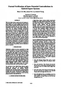
timers can be found in PLCs, one of the most common timers is TON (Timer On-delay) (see Fig. 1). This timer has 2 inputs variables: IN and PT. IN is a Boolean input signal and PT is the delay time. The timer has 2 outputs: Q and ET. Q is the Boolean output variable, its value will be true after the predefined delay (PT ) when IN performs a rising edge, and it will be false if IN is false. ET is the elapsed time, its value is increased until PT, starting when a rising edge occurred on IN. 1
IN input
0 1
Q output
ET
PT
0
PT
elapsed time
0
t
Fig. 1. TON time diagram PLC timers use a specific data type for timing operations called TIME. This data type is defined by IEC 61131 as a finite variable which states that “The range of values and precision of representation in these data types is implementation-dependent”. Representing time by a finite variable leads to a non-monotonic time representation as the variable can overflow (c.f. the upper part of Fig. 3). For example, in Siemens S7 PLCs, the TIME data type is defined as a signed 32-bit integer with the same precision of 1 ms (see Siemens (1998)), having an upper limit of approximately +24 days and a lower limit of −24 days. However, in Schneider and Beckhoff PLCs, the TIME data type is an unsigned 32-bit integer with a precision of 1 ms. In this paper, we consider the signed time interpretation as defined in Siemens PLCs.
2.2 Case study In the context of this paper, the industrial control system framework, developed and used by CERN, called UNICOS (Blanco et al. (2011)) is taken as a case study. UNICOS provides a library of base objects representing common industrial control instrumentation (e.g. sensor, actuators, subsystems). These objects are represented as function blocks in the PLC code, using the ST (Structured Text) language, which can call different functions, function blocks on the PLC. Currently UNICOS is implemented for standard PLCs, i.e. in which the cycle time is not fixed and depends on the overall application. In this paper, we focus on the OnOff object provided by the UNICOS library for Siemens PLCs. This object is used to represent a physical equipment, as actuators driven by digital signals (e.g. valves, heaters, motors). With 60 input variables (of which 13 are parameters), 62 output variables, 600 lines of ST code, and 3 timer instances, the OnOff object is representative of other UNICOS objects in terms of size and complexity.
3. MODELLING PLC PROGRAMS This section gives a brief overview of the general methodology for modelling PLC programs without considering timing aspects. For more details, readers should refer to Darvas et al. (2013). Also, the applied reductions and abstractions are introduced. 3.1 Methodology This methodology aims to generate formal models out of ST code. It provides an intermediate model and a set of transformation rules to produce the input models for different verification tools from the “non-formal world” of control systems (see Fig. 2). This “non-formal world” is basically composed by the ST program and environmental factors related to the execution platform (for example the PLC scan cycle). ST code IF c THEN s1; ELSE s2; ...
abstractions / reductions intermediate model
• General rule-based reductions are used to simplify the generated automata by taking advantage of the characteristics of the PLC’s execution model. For example, variable assignments on succeeding transitions can be merged if they are not affecting each other, as the value of the variables are not checked during the execution of the PLC cycle but only at the end. More than 20 rules have been defined to simplify and reduce the model. • When the property to verify is provided, we apply the Cone of Influence (COI) reduction (c.f. Clarke et al. (1999)), which consists in removing all variables that do not affect the property. As it is depending on the requirement to be checked, its impact on the size of the state space highly varies, but for many examples, we can observe a large state space reduction. • In some cases, predicate abstraction can be also applied to PLC applications. It consists in substituting non-Boolean variables by Boolean-valued functions.
NuSMV model next(loc) := case loc = s & c: s1; loc = s & !c: s2; ...
Model checking
The reader find detailed information about the applied techniques in Darvas et al. (2014).
s [c]
PLC environment
s1
t1
t2 [NOTwc]
Non-formalwworld
BIP model
s2
UPPAAL model
–wcyclicwbehaviour –wconstantwinputs duringwthewcycle –w...
Simulation
... Intermediatewmodel
Formalwmodels
Verification
Fig. 2. Overview of generic methodology producing formal models out of ST code. This intermediate model based on automata simplifies the transformation rules to any formal model used by a model checker, whose modelling language is close to an automata-based formalism. It allows to easily add new model checkers to the methodology and verify the same model with different verification tools, thus benefiting from the different advantages of the verification tools in terms of verification performance, simulation and expressiveness of properties specification. Our automata-based formalism is strong enough to model all relevant features of a PLC control system. The semantics of the intermediate model is similar to the network of timed automata formalism defined in Behrmann et al. (2004) but without explicit logical clock representation. In addition, an automatic generation tool has been developed supporting this methodology, which allows to generate models for NuSMV, UPPAAL and BIP out of ST code. 3.2 Reduction and abstraction techniques Modelling PLC programs for verification purposes implies the creation of models with huge state spaces, as it happens for any other real-life software. If these are timed systems, then modelling of time is required, so the problem becomes even bigger. Although the main goal of this paper is not to present the abstraction techniques applied on the generated models in details, we introduce them as they are needed to understand our experimental results on timed PLC programs. These techniques are included in the methodology and applied automatically to the intermediate model, therefore all the generated final models benefit from them. The main abstraction and reduction techniques applied:
4. MODELLING TIMING ASPECTS OF PLC PROGRAMS This section focuses on the modelling aspects of PLC time and timers extending the described methodology in Section 3. The TON timer, presented in Section 2, is used to illustrate the two proposed approaches to model timing aspects, but the same methodology can be applied to any other PLC timer block. In the proposed methodology extension, a PLC timer is represented by a separated automaton which is synchronized with the main program. Modelling PLC timers also implies to model the TIME data type. However, as mentioned previously, timed models usually contain a huge state space, which cannot be handled by model checkers. Based on this observation, two different approaches are proposed in this section. The first is a realistic timer representation, which is close to the reality, enabling precise modelling and verification. The second approach proposes an abstract time representation, which is less accurate, but drastically reduces the state space of the model. Both approaches are analyzed hereafter paying attention to time and timer representation, property specification, and experimental results. In addition, we are presenting the proof that the abstract approach simulates the realistic one, thus guaranteeing that any property verified by the abstract approach also holds in the realistic one, even if is much simpler. 4.1 Realistic approach This first approach presents a realistic model of a TON timer and the time handling. This approach allows to specify properties with explicit time in it. Having this realistic representation of the timer implies that time needs also to be modelled realistically. Time representation Three main characteristics are considered to model time for this approach:
(1) Time is modelled as a finite variable: it represents with high fidelity the TIME data type in a PLC. However, instead of having a signed 32-bits integer variable (like in Siemens PLCs), a 16-bits variable is used to represent this data type. This range reduction is possible as the behaviour of a PLC is cyclic and the cycle time, the delays of the timers, and the delays in the requirements are much smaller than the range of this 16 bit variable. The accuracy of this variable is 1 ms, as it is in real PLCs. Because of this time representation, overflow of time has to be considered when the timer is modelled, also when the requirement to be checked is expressed (e.g., the current time can be smaller for a later event, see Fig. 3). (2) Time is incremented by adding the cycle time: In this representation, time is not incremented by individual units of time. It is instead incremented by the duration of the last PLC cycle at the end of it. This assumption obviously simplifies the global model and there is not any loss of accuracy when comparing with the real implementation in a PLC, considering that the timers are called at most once in each PLC cycle, which holds for our real cases.
current time (ctime)
(3) Cycle time is chosen non-deterministically: in order to represent standard PLC with a varying cycle time, a random value is generated at the end of each cycle to represent this. The selected random values are between 5 ms and 100 ms, which is a valid assumption based on the PLC systems at CERN. max. TIME
IF in = false THEN Q := false; ET := 0; running := false; // ELSIF running = false THEN start := CTIME; running := true; // ELSIF CTIME - (start + PT) >= 0 THEN Q := true; ET := PT; // ELSE IF not Q THEN ET := CTIME - start; END_IF;
t2 t3 END_IF;
Only one transition can happen in this state machine for every call of the timer. Therefore the timer cannot go from state NR to state TO with one function call, which is valid if we assume that delays are always greater than zero (PT > 0). According to the specification of the Siemens TON implementation (Siemens (1998)), the parameter PT should be positive. The potential state space (PSS) size of this timer representation is 3.38 · 1016 and its reachable state space (RSS) is 5.91 · 1015 without counting the variable ctime (as it is a global variable used by all the timers). [¬in]
NR t1
[in] / start:=CTIME
running=false Q=false
t1
t1
[¬in]
[¬in]
t2
tm
t
running=true Q=false
TO t4
[in ∧ P]
[in ∧ ¬P]
min. TIME
// t4
Fig. 4. ST code of TON
R
0
t1
t3
running=true Q=true t3
t4
[in ∧ ¬P]
[in ∧ P]
P ≡ (CTIME − (start + P T ) ≥ 0)
tm start time < stop time
Fig. 3. Consequences of finite time representation Timer representation Given this finite time representation, the behaviour of the timer is represented as it is shown on the ST code (see Fig. 4). In this code, the input variables are IN and PT, and the output variables are Q and ET. The variable ctime represents the current time and it is modelled as previously explained. In addition, two variables are added: running and start, where running is a Boolean variable representing when the timer is working after a rising edge on IN and start contains the value of ctime when IN has a rising edge. By applying the extended methodology, the corresponding automaton of the TON ST code was produced and the equivalent state machine is shown in Fig. 5. (Note that the assignments of ET are omitted from the state machine to simplify the figure.) This state machine contains 3 states corresponding to the 3 original states of the TON: NR (not running; running=false, Q=false), R (running; running=true, Q=false) and TO (timeout; running=true, Q=true). The transitions in the state machine (labelled as t1 , t2 , t3 , t4 ) correspond to the conditional statements in the ST code.
Fig. 5. State machine of the realistic TON representation Property specification Using the methodology and the developed tool, input models for NuSMV are automatically generated. The experimental results presented here are produced using this model checker. NuSMV provides CTL (Computational Tree Logic) and LTL (Linear Temporal Logic) for property specification. Our goal is to verify properties with explicit time in it, like “if C1 is true, after tm time C2 will be true, if C1 remained true” (where C1 and C2 are Boolean expressions, C1 contains input variables and parameters and C2 contains output variables). CTL and LTL do not provide this expressiveness, for this reason a monitor or observer automata is added to the model. The goal of the monitor is to check C1 , and if it is true for at least tm time, the monitor output value Mout is set to true. By using such monitor, the requirement is simplified as “if Mout is true, then C2 should be true”. This requirement can be formalized easily in CTL: AG(Mout → C2 ). An example for this monitor usage can be seen on Fig. 6. As the computed values are assigned to the real outputs of the PLC only at the end of the PLC cycle, the requirements should be checked only at this point. The general CTL expression extended with it is the following: AG(PLC END → (Mout → C2 )), where PLC END is true, iff the execution is at the end of a PLC scan cycle.
fixed parameters
The behaviour of this monitor is similar to the TON timer, but it is independent of the rest of the program logic, therefore Mout will be true after tm time, if C1 is true and it can be used to verify if outn holds the property. It has to be noticed, that it is not enough to save a “timestamp” tC1 when C1 is true, and formalize the requirement as AG((ctime ≥ tC1 + tm ) → C2 ), because the ctime variable is a finite integer, thus it can overflow, as it is illustrated by Fig. 3. outputs par1
10 s (tp)
out1
OnOff
the maximal cycle time, 100 ms in this case, because the current time is incremented in quanta. Table 1. State space of the OnOff model with realistic time representation Time 32 bit 16 bit 16 bit 16 bit 16 bit 16 bit
Monitor – – – + + +
Reductions none none general general general, COI gen., fix params, COI
PSS 1.6 · 10218 2.5 · 10160 1.6 · 10134 8.5 · 10139 1.1 · 1085 1.1 · 1036
#Vars 255 255 185 189 143 86
...
false
PT
Q
TON
IN
logic
logic
inputs
Table 2. Verification time on OnOff model with realistic time representation
...
in1 in2
outn compare
inn
monitor enabled
10 s (tm)
if Mout is true, outn should be true also
Mout
delay
Fig. 6. Verification configuration for OnOff model extended with monitor Experimental results This approach has been applied to the UNICOS framework. In particular, the experiments showed here have been applied to the OnOff object from the UNICOS library. Table 1 presents different state spaces depending on which abstraction and reductions techniques are applied. On the OnOff model, we made our experiments with a requirement of the previously introduced structure: “if C1 is true, after tm units of time C2 will be true, if C1 remained true”. To be able to verify this property, the original model was shrink from a PSS of 1.6 · 10218 states to a PSS of 1.1 · 1036 as can be seen in Table 1. In order to do so, reductions, fixed parameters (focusing on a specific scenario), and COI technique (which eliminated 2 timers out of 3) have been applied. As it was mentioned before, time values were modelled as 16-bits variables instead of 32-bits. Table 2 presents verification results for the OnOff model after applying all the previously mentioned reduction techniques. We checked the introduced requirement with three different configurations in terms of timer delay (tp ) and monitor delay (tm ). The first uses tp = tm = 10 s values, which means the parameter tp of OnOff and the delay parameter tm of the monitor were both 10 s. In this case, the result is true which is given by NuSMV in 11.4 s. The other two configurations use monitor delay times smaller than the parameter tp , therefore the output is expected too early, thus the result should be false. As it can be seen in Table 2, in both cases the verification time was around 5–20 s, but the generation of the counterexample (C.ex. gen. time) took significantly more time. In the case when we used tm = 9 s, the counterexample was longer (3 876 steps), and its generation time was around 15 times bigger than when we used tm = 1 s. Notice that these verification results can have a timing error not bigger than
Timer delay (tp ) 10 s 10 s 2s
Monitor delay (tm ) 10 s 9s 1s
Result true false false
Run time 11.4 s 19.5 s 5.2 s
C.ex. gen. time — 2513.2 s 123.0 s
C.ex. length — 3 876 510
4.2 Abstract approach As it was shown in the previous experimental results, the models created by realistic approach have a big state space even if only one TON is modelled. If this approach is applied to larger models than the UNICOS OnOff object probably verification would not be even possible. For that reason, we propose a second approach based on a data abstraction of the first approach. Time representation In this case, time is not represented explicitly in the model, the variable ctime representing the current time is not maintained. Therefore properties with explicit time cannot be validated. Timer representation This timer representation approach consists in a non-deterministic model produced as an abstraction of the realistic approach. The corresponding state machine is presented in Figure 7. Similarly to the realistic model, this model has three possible internal state: NR (not running), R (running) and TO (timed out). If the input IN is true, the TON will start to run (goes to state R). After that, the TON can stay in the state R or go to TO non-deterministically, which means, we do not know when the timer will stop. However, by adding a fairness constraint to the model, it is ensured that the timer cannot stay in state R for infinite time. In one PLC cycle only one transition can be fired, i.e., the timer cannot go from state NR to state TO with one call. This corresponds to the previously introduced PT > 0 constraint. Figure 8 shows the timing diagram of the abstract approach compared with the realistic one. The size of the PSS and RSS for this model is 6 comprising the Boolean input variable, reducing significantly the size of the realistic approach but introducing some limitations of the property specification. This representation can result false positives, meaning that verification tools can give spurious counterexample that cannot occur in reality. However false negatives can never occur, therefore if a property holds in the abstract model, it holds in the real system.
Table 3. State space of the OnOff model with abstract time representation
[¬in] NR Q=false
[in]
Reductions none general general, COI, fix params (Exp. 1) general, COI (Exp. 2, 3)
[¬in] [¬in]