WETLANDS, Vol. 28, No. 2, June 2008, pp. 336–346 ’ 2008, The Society of Wetland Scientists
MONITORING MANGROVE FOREST CHANGES USING REMOTE SENSING AND GIS DATA WITH DECISION-TREE LEARNING Kai Liu1, Xia Li2, Xun Shi3, and Shugong Wang4 Guangzhou Institute of Geochemistry, Chinese Academy of Sciences Guangzhou, P.R. China, 510640 Guangzhou Institute of Geography Guangzhou, P.R. China, 510070, and Graduate School of Chinese Academy of Sciences Beijing, P.R. China, 100049
1
2
School of Geography and Planning, Sun Yat-sen University Guangzhou, P.R. China, 510275 E-mail:
[email protected] 3
Department of Geography, Dartmouth College Hanover, New Hampshire, USA 03755 USA
4
Institute of Environmental Science, Sun Yat-sen University Guangzhou, P.R. China, 51027
Abstract: This paper presents a decision-tree method for identifying mangroves in the Pearl River Estuary using multi-temporal Landsat TM data and ancillary GIS data. Remote sensing can be used to obtain mangrove distribution information. However, serious confusion in mangrove classification using conventional methods can develop because some types of land cover (e.g., agricultural land and forests) have similar spectral behaviors and distribution features to mangroves. This paper develops a decisiontree learning method for integrating Landsat TM data and ancillary GIS data (e.g., DEM and proximity variables) to solve this problem. The analysis has demonstrated that this approach can produce superior mangrove classification results to using only imagery or ancillary data. Three temporal maps of mangroves in the Pearl River Estuary were obtained using this decision-tree method. Monitoring results indicated a rapid decline of mangrove forest area in recent decades because of intensified human activities. Key Words: change detection, DEM, Landsat TM image, Pearl River Estuary
Province, where more than half of the mangrove forests in China are located, two-thirds of them have vanished in the past two decades (Wang and Chen 1998). Declines of mangrove forests are mostly due to massive reclamation projects in the coastal regions, destruction by tidal waves, and rapid urbanization (Linneweber and de Lacerda 2002). Mapping and monitoring of mangrove forest decline has become an urgent need for many countries (Jensen et al. 1991, Ramsey and Jensen 1996, Gao 1999, Vanina et al. 1999, Munyati 2000, Proisy et al. 2000, Kovacs et al. 2001, 2005, Li et al. 2002). Many studies indicate that remote sensing has advantages over traditional field investigation methods in monitoring of wide-spread mangroves (Sader et al. 1995, Brian and Timothy 1996, Green et al. 1998, Kovacs et al. 1999, 2005, Akira et al. 2003,
INTRODUCTION Mangroves are small evergreen trees that flourish in the intertidal zones of river deltas, lagoons, estuaries, and coastal systems in the tropics, subtropics, and some temperate coasts (Twilley et al. 1996, Sheridan and Hays 2003). Mangroves provide a variety of ecological services for human beings, such as the protection of coasts from typhoon damage, pollutant absorption, and water purification. They are also habitats for a diverse flora and fauna, including many rare species (Blasco et al. 1996, Murray et al. 2003, Sheridan and Hays 2003). However, about one-third of mangrove forests have been lost within the past 50 years worldwide (Alongi 2002). Drastic declines have also occurred in China. For example, in the Guangdong 336 Wetlands wetl-28-02-07.3d 21/3/08 14:56:29
336
Cust # 06-91
Liu et al., MONITORING MANGROVE CHANGES Hirano et al. 2003). Remote sensing technology can obtain information about inaccessible areas and extreme environments (Vaiphasa et al. 2006). A number of satellite sensors have been used to identify mangrove forests, including TM/ETM (Brian and Timothy 1996), SPOT (Franklin 1993, Pasqualini et al. 1999), CBERS (Li et al. 2002), SIR (Pasqualini et al. 1999), ASTER (Vaiphasa et al. 2006), and IKONOS and QuickBird (Wang et al. 2004). Many such studies, however, are primarily based on supervised classifications (Sader et al. 1995, Pedro et al. 1998, Wang and Chen, 1998, Munyati 2000, Li et al. 2002, Wang et al. 2004). For example, Garcia et al. (1998) assessed mangrove vegetation in Mexico’s Santiago River Mouth by applying supervised classification to Landsat TM imagery. Pasqualini et al. (1999) used SPOT-XS and SIR-C radar data and a supervised classification method to map mangrove forests of Madagascar. Wang et al. (2004) used meter-level satellite imagery (IKONOS and QuickBird) and a maximum likelihood classification (MLC) method to distinguish different species of mangrove forest on Panama’s Caribbean coast. Supervised classification is a common method for interpreting remote sensing data, but it heavily depends on the user’s skill and training, and often requires time-consuming analysis. Machine learning techniques have been increasingly used in remote sensing applications related to wetlands research (Huang and Jensen 1997, Horssen et al. 2002, Colstoun et al. 2003). Recent research has demonstrated that the decision tree, one of the most popular machine learning approaches, can be accurate and efficient in land cover classification based on remotely sensed data (Swain and Hauska 1977, Hansen et al. 1996, Friedl and Brodley 1997, Defries et al. 1998, Friedl et al. 1999). The decisiontree learning algorithm can create classification rules directly from the training data without human intervention. In addition, unlike many other statistical analysis approaches, such as maximum likelihood classification, the decision tree does not depend on assumptions about value distribution or the independence of the variables from one another (Quinlan 1993). This is important for incorporating ancillary GIS data, because they usually have various value distributions and may be highly correlated (Jensen 2005). Rule sets can be applied to classification of multi-temporal images after they have been acquired from decision-tree learning. Using the same rule sets can ensure the classification results are comparable between different temporal images, which should be more advantageous than traditional methods for monitoring mangrove forest change from time series of remote sensing data.
Wetlands wetl-28-02-07.3d 21/3/08 14:56:37
337
Cust # 06-91
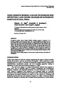
337 This study explores the applicability of the decision-tree learning method in detecting rapid changes in the mangrove forests in China’s Pearl River Estuary based on an integration of multitemporal Landsat TM data. We applied the rule set derived from the data of 2002 to the data of 1988 and 1995, in order to detect change of the mangrove forests over the period. We anticipated that the decision-tree method would be able to improve the performance mangrove forest monitoring with multitemporal Landsat TM images and GIS ancillary data. METHODS Decision-Tree Algorithm A decision tree is a classification procedure that recursively partitions a data set into smaller subsets based on a test defined at each branch (or node) of the tree. The tree is composed of a starting node (root), a set of internal nodes (splits), and a set of terminal nodes (leaves). Except the root, each node has one parent node; and except leaves, each node has two or more descendant nodes (Friedl and Brodley 1997). Through the tree, the observations are sequentially divided by the tree, and each observation will be finally assigned a class label according to the leaf node it reaches (Breiman et al. 1984, Quinlan 1986, Xu et al. 2005). A number of algorithms are available for decision-tree learning, including ID3 (Quinlan 1986), C4.5 (Quinlan 1993), and CART (Breiman et al. 1984). C4.5 (Quinlan 1993) is the first inductive decision-tree learning program and has been widely used (Mulholland et al. 1995, Berry and Linoff 1997). C5.0 for UNIX and its Windows counterpart See5 are the most updated versions of C4.5. See5 is the program adopted by this study. The procedure of applying See5 includes construction of the training set, training of the decision-tree, and translation of the decision tree to rules (Quinlan 1993, Jensen 2005). The training set consists of a set of samples for which we know both their attribute values and the classes to which they belong. Each sample is represented by an attribute-class vector: [ID_j, Attribute_1, Attribute_2, … , Attribute_n, class_i] (Quinlan 1993). The training set is used to train the decision tree, i.e., determine the attribute and threshold at each node. The most widely used method for this determination is the ‘‘information gain ratio’’ from communication theory, which selects the attribute with the minimum entropy to be the ‘‘splitting’’ attribute (Quinlan 1993). Figure 1A shows an example of a trained decision tree. In this figure, observation set T is first divided into
338
WETLANDS, Volume 28, No. 2, 2008
Figure 1.
A) A hypothetical decision tree with B) Examples of classification rules.
subsets T1 and T2 according to the value of attribute A1. Next, set T1 is divided into subset T3 and class d according to the value of attribute A2. This process continues until all subsets find their classes (the leaf nodes). The decision tree in Figure 1 has A1 as the attribute at the root node, and A2, A3, and A4 as the attributes at the split nodes. The branches for T1, T2, and T3 can be considered as sub-trees. A decision tree is often too complex to understand, especially when it is large. In practice, people often translate a decision tree to other representations of knowledge, such as classification rules (Jensen 2005). Classification rules are normally in the form of ‘‘IF condition, THEN action’’ statements. The condition portion of a classification rule is usually a fact (e.g., Attribute-1 . 10 and Attribute-2 # 20), and the action portion is usually a decision (e.g., class label 5 a). For a decision tree, each path from the root node to a leaf node can be translated into a classification rule. In the example illustrated by Figure 1A, the paths from the root node to the leaf nodes b, d, and a can be translated to classification rules listed in Figure 1B. A problem often encountered in a decision-tree process is overfitting. The training process can overly fit the tree to the training set, which results in redundancy of information and error in actual classifications, particularly when the training data contain errors (Mingers 1989, Friedl et al. 1999). A ‘‘pruning’’ method deals with such problem by removing parts of the tree. The general process of pruning is to replace a sub-tree by a leaf or subbranch to see if this will improve the performance of the tree as a whole. See5 provides functions to perform such pruning.
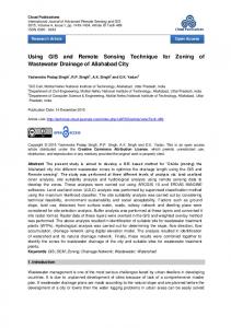
and 113u319120 – 114u49400 E (Figure 2). Various geomorphologic habitats are present in the area, including muddy beaches, sandy beaches, and rocky beaches along the coast. A variety of mangrove species occur in the area, providing a favorable habitat for numerous marine and terrestrial plants and animals. The region has also become densely populated and intensively developed, which has significantly impacted the local ecology. Monitoring of mangrove forests was based on three temporal Landsat TM images, including the scenes at path 122 and row 44 with acquisition dates of December 10, 1988, December 30, 1995, and November 7, 2002. They were obtained as radiometrically corrected (level 1G) data in digital number (DN) values. The DEM data and coastal information from GIS were also used as input attributes to the See5 system. Tidal information was collected for the reference dates. Image pre-processing includes radiation correction and geometric rectification. Both absolute and relative radiation corrections were performed. This
STUDY AREA AND DATA SOURCES The study area is the Pearl River Estuary, with spatial extent defined by 22u209490 – 22u559520 N
Wetlands wetl-28-02-07.3d 21/3/08 14:56:37
338
Cust # 06-91
Figure 2.
The study area in the Pearl River Delta.
Liu et al., MONITORING MANGROVE CHANGES
339
Table 1. Tide data for three temporal images of Pearl River Delta. Data source: The observatory station of Lingding Island. December 10, 1988 Time
December 30, 1995
Height (cm)
Time
05:23 46 12:24 190 15:54 161 22:26 320 Tidal height for the image 169 cm
Mangroves Agricultural land Forests Surface water Urban areas Fallow land
Description Mangrove forests Crop fields, pastures, and grasslands Deciduous or evergreen forest land, orchards, and tree groves Permanent open water, lakes, reservoirs, bays, and estuaries Residential, commercial, industrial, and other developed land Fields no longer under cultivation
Wetlands wetl-28-02-07.3d 21/3/08 14:56:39
339
Time
Height (cm)
05:55 58 12:38 200 17:10 147 23:38 310 Tidal height for the image 172 cm
Jensen 2005 on rectifying Landsat TM imageries, the rectification in this study used a first-order polynomial model. Resampling used the nearest neighbor algorithm to maintain the geometric integrity of the data (Rutchey and Vilcheck 1994, ERDAS 1997, Harvey and Hill 2001, Campbell 2002). The average root mean square error (RMSE) is about 0.5 pixels. The software used for the pre-processing of Landsat TM images was ERDAS Imagine. Ideally the acquired remote sensing images all have similar tidal heights so that the classification results can be better compared. Luckily, based on the available tidal information (Table 1), the three images used in this study had very similar tidal heights. Besides mangrove forests, other major land cover types in the Pearl River Estuary were also identified from the three Landsat TM images using the decision-tree method. This provided context information about mangrove forest dynamics. Table 2 lists all six land cover types identified by the decision tree: 1) mangroves, 2) agricultural land, 3) forests, 4) surface water, 5) urban areas, and 6) fallow land. To improve classification accuracy, especially to reduce misclassification between mangrove forest and agricultural land, we implemented a two-step procedure. The first step only identified mangrove forests, and the second step classified the other nonmangrove land cover types (Figure 3). APPLYING A DECISION TREE LEARNING METHOD
Land-cover classification scheme.
Land-cover class
Height (cm)
03:01 61 09:32 194 14:08 138 20:28 300 Tidal height for the image 183 cm
kind of correction is required for applying the classification rule set derived from one image to the other two. Absolute radiation correction is a model of correcting (such as 6S model) that translates pixel values to radiance and is used in remote sensing inversion. Relative radiation correction means that the pixel value was related to relative digital number levels without units. Many studies have shown that these corrections are useful in classification and monitoring of land cover changes (Song et al. 2001, Vogelmann et al. 2001, Li et al. 2004, Olthof et al. 2005, Roder et al. 2005). Simple histogram matching was used in this study for relative radiation correction. Histogram matching is conceptually similar to histogram equalization, which stretches pixel values of an image to match a standard range. It can use one image as the standard and matches all other images of concern to the range of that image. While simple, this method has proved to be effective for relative radiation correction (Richards and Jia 2006). In this study, the histograms of the 1988 and 1995 TM images were translated to the range of the 2002 TM image. The images were then rectified to spatially match the GIS maps using ground control points (GCPs). A total of 50 GCPs were interactively selected across the entire area of each image. Most GCPs were intersections of roads and rivers that could be easily identified, and the points had a largely even distribution. Referring to Jensen et al. 1988 and Table 2.
November 7, 2002
Cust # 06-91
The process of applying the decision-tree method to multi-temporal Landsat TM images and ancillary GIS data for detecting the temporal changes of mangrove forests in the Pearl River Estuary is summarized by Figure 4. Generating Classification Rules Using See5 In the decision-tree learning approach, remote sensing images (i.e., bands) and ancillary GIS data
340
WETLANDS, Volume 28, No. 2, 2008 NDVI was calculated as follows (Adams et al. 1995, Hansen and Schjoerring 2003, Mather 2004): Band4{Band3 ð1Þ Band4zBand3 In many places, rules solely based on the TM data would not be able to distinguish mangrove forests from non-mangrove forests. In this study, two attributes, elevation and distance to coastline, based on the data from existing GIS databases and field investigations, were used to improve the accuracy of the classification. Mangrove forests are constrained by topographic factors. Field investigations found that mangrove forests were not distributed above 10 m elevation. Therefore, the digital elevation model (DEM) was used to exclude non-mangrove pixels that had similar spectral attributes with mangrove pixels, but were above the elevation limiting line. Field investigation also found that mangrove wetlands are unlikely to be found beyond 1 km from the coastline. To incorporate this information, coastlines were first identified using TM images, and then the distance from each pixel to the coastline was calculated using the Eucdistance function of ARC/INFO GRID (Li and Yeh 2004). Table 3 lists the attributes used in this study for generating the decision tree. NDVI~
Figure 3. Classification of mangrove forests versus other land-covers in the Pearl River Delta.
are used as attributes, while the types of land cover (i.e., mangrove, non-mangrove) define the class labels. Attributes are associated with the root node and split nodes of the decision tree, while class labels are associated with the leaf nodes. The following process was implemented using See5. Preparing the Sample Set and Determining Attributes In this study, the sample data set was obtained by classifying a total of 1,000 pixels based on field investigation of the year 2002 TM image. The sample set was divided into two groups: 1) 80% of the samples were used as the training set and 2) the others were put into a test set. The training set was used to train and construct the decision tree, and the test set was used for testing the accuracy of the constructed tree. The attributes of the samples fell into two categories: 1) remote sensing data, including the original values of each TM bands and the NDVI value and 2) GIS data, including elevation, proximities to the coastline, and spatial locations (coordinates). The class label has two possible values: mangrove forest is represented by C1 and nonmangrove is represented by C2. The seven bands of TM data were the basic attributes used for the classification. Normalized Difference Vegetation Index (NDVI) was also included as one of the major attributes for representing vegetation conditions. For TM images,
Wetlands wetl-28-02-07.3d 21/3/08 14:56:39
340
Generating a Decision Tree and Transforming to Rules With See5, the decision tree and classification rules could be generated automatically from the samples. However, an important parameter, the pruning rate, needed to be assigned before executing the automatic process. In this study, a pruning rate of 25% was used to address the trade-off between classification accuracy and decision-tree size. Figure 5 is the decision tree model generated from See5. Some examples of the classification rules translated from this tree are shown by Figure 4. Table 4 shows the error for the training and test data. For both sets, the generated decision tree had accuracies . 90%. Identifying Temporal Change in Mangrove Forests using the Classification Rules The extracted classification rules were applied to the TM images from 1988, 1995, and 2002 (Classification section in Figure 4). The classification of mangrove and non-mangrove pixels based on these rules was conducted using the ERDAS IMAGINE’s Knowledge Engineer and Knowledge Classification tools. Classification results for the
Cust # 06-91
Liu et al., MONITORING MANGROVE CHANGES
Figure 4.
Flow chart for monitoring mangrove forests in the Pearl River Delta.
three years were overlaid to detect mangrove change.
distribution. However, our study shows that distance to coastline and elevation by themselves were not deterministic in identifying mangrove forests, since different land cover types can occur in places that are otherwise similar in terms of these two factors. Figure 6g and 6h show the results from decision trees that only used these two factors as attributes. Satellite image data usually accurately
Effect of Incorporating Ancillary GIS Data Mangrove forests require a special ecological environment, making the data on distance to coastline and elevation useful in delineating their Table 3.
341
Attributes used for the See5 system. Attributes
1. Spectral attribute (TM bands 1–5, 7, and NDVI) 2. Elevation attribute (DEM) 3. Distance attribute (Distance to the coastlines) 4. Spatial attribute (longitude and latitude of sampling pixel)
Wetlands wetl-28-02-07.3d 21/3/08 14:56:40
Acquisition methods
Value range
Samples from TM image and NDVI image in ARC/INFO GRID Samples of DEM image in ARC/INFO GRID Eucdistance of ARC/INFO GRID
TM bands: 0–255 NDVI: 21–1 DEM: 0–500 (integer) Distance: 0–20 km
Field investigation
yyuyy9yy0
341
Cust # 06-91
342
WETLANDS, Volume 28, No. 2, 2008
Figure 5. The decision tree generated using the See5 computer program.
distinguish vegetation from other land cover types such as urban and surface water. However, separating mangrove forests from other types of forests can be difficult if only spectral data are used (Figure 6i). An integration of the two types of data generates considerably better results (Figure 6j). Classification of Other Land Cover Types Areas that were not mangrove forests were first extracted by applying the Mask function in ERDAS. The land cover types in these areas, including agricultural land, forest, surface water, urban etc., were then identified using the decision tree method. To simplify the procedure, only spectral data were used as the attributes for the decision tree in identifying these land cover types. Base on the analysis of the spectral characteristics of these land cover types (Figure 7), seven attributes from the TM data, including band1, band2, band3, band4, band5, Table 4. The accuracy of the decision tree method for detecting mangrove trees. N 5 number of samples in each class; C1 5 mangrove; C2 5 non-mangrove.
Class Code Name 1 2
C1 C2
Training Data (800)
Test Data (200)
C1
C2
Error
C1
C2 Error
196 142 804 24
12 622
4.5%
38 9
5 7.0% 148
N
Wetlands wetl-28-02-07.3d 21/3/08 14:56:41
342
Figure 6. a-f) Image data and ancillary GIS data used to identify mangrove forest on the area of Shenzhen River in the Pearl River Estuary; g) Classification only using the proximity variable; h) Classification using both the proximity variable and the DEM data; i) Classification using the spectral data; j) Classification using the proximity variable, the DEM, and the spectral data.
Cust # 06-91
Liu et al., MONITORING MANGROVE CHANGES
Figure 7.
Spectral characteristics of non-mangrove land-covers using TM images.
Figure 8.
Land cover type classification maps of the Pearl River Estuary.
Wetlands wetl-28-02-07.3d 21/3/08 14:56:45
343
Cust # 06-91
343
344
Table 5.
WETLANDS, Volume 28, No. 2, 2008
Change in mangrove forests and other land-covers from 1988 to 1995 to 2002. 1988
1995
2002
Land-cover
ha
%
ha
%
ha
%
Mangroves Surface water Forest Agricultural land Urban area Fallow field
473 157,380 114,350 52,705 13,959 25,274
0.13 43.22 31.40 14.47 3.83 6.94
303 154,258 98,503 46,549 25,652 38,875
0.08 42.36 27.05 12.78 7.04 10.68
427 15,2021 118,033 37,300 31,849 24,510
0.12 41.75 32.41 10.24 8.75 6.73
band7, and NDVI, were selected as the inputs for the decision tree. A total of 3,000 samples were collected to construct the sample set, of which 2,000 were used as the training samples and the remaining 1,000 formed the test set. The resulting decision tree had errors of 15.9% and 20.7% for the training and test sets, respectively, both higher than their counter parts in the identification of mangrove forests, apparently due to lack of the controls enforced by the ancillary GIS data. Still, the decision tree led to a highly complicated classification system containing 87 rules. This system was applied to the images from the three different years and results were used to detect land cover change (Figure 8). Results of Change Detection Details of the detected change of mangrove forests and other land-covers in the study area are summarized in Table 5. According to our results, mangrove forests were extensively distributed in the coastal area of the Pearl River Estuary throughout the study period. There was a significant decrease from 1988 to 1995, and then a slight increase from 1995 to 2002. Generally, the total area of mangrove forests was declining (a reduction of 45.8 ha from 1988 to 2002) and fragmentation was obvious. Field investigations have shown that most wild mangrove forests have been lost in the Pearl River Delta. Only those contained in natural reserves have been well protected. Human-planted mangrove forests have largely replaced wild ones. Other forests in the area had a similar trend over the study period. Except for Table 6.
1988 1995 2002
fallow land, changes in the other non-forest types were linear. Specifically, urban areas continually expanded, while the agricultural areas and surface water continually shrank. The fallow land showed an increasing-decreasing pattern. Classification Assessment To assess the accuracy of the classification results from the decision trees, we first conducted field sampling and then used the ground truth to build error matrices. The field sampling adopted a stratified random sampling so that the distribution of the sample points was relatively even across different land cover categories (Congalton 1991). Besides the correctness for each category that can be directly read from the error matrix (Hord and Brooner 1976, Congalton 1991), we also calculated more sophisticated Kappa coefficients to measure differences between actual and chance agreement (Cohen 1960, Fung and LeDrew 1988, Congalton 1991, Campbell 2002). The error matrices for the three years and their corresponding Kappa values are listed in Table 6. It was not surprising that results of 2002 had the highest accuracy because the TM image from this year was used to build the decision tree. However, we consider the results from the other two years to also be satisfactory. Their relatively high accuracies indicate that a decision tree built using the data from one year may be reused for other years in identifying mangrove forests. As a result, we might be able to establish a general classification rule set for this application.
Error matrix of decision tree classification in 1988, 1995, and 2002. Non-mangrove
Mangrove
Total Accuracy
Kappa coefficient
218 63 215 43 224 38
32 187 35 207 26 212
81.0%
0.74
84.4%
0.77
87.2%
0.81
Non-mangrove Mangrove Non-mangrove Mangrove Non-mangrove Mangrove
Wetlands wetl-28-02-07.3d 21/3/08 14:56:51
344
Cust # 06-91
Liu et al., MONITORING MANGROVE CHANGES In summary, this work demonstrates that the use of the decision-tree method on a combined dataset containing multi-temporal TM images and GIS data can be effective in delineating spatial distribution and temporal change of mangrove forests. Further studies should be carried out to integrate various sources of remote sensing data to discern different types of mangrove forests. ACKNOWLEDGMENTS This study was supported by the National Outstanding Youth Foundation of China (Grant No. 40525002), the National Natural Science Foundation of China (Grant No. 40471105), and the Outstanding Youth Foundation of Guangdong Academy of Sciences (2008). LITERATURE CITED Adams, J. B., D. E. Sabol, V. Kapos, R. A. Filho, D. A. Roberts, M. O. Smith, and A. R. Gillespie. 1995. Classification of multispectral images based on fractions of endmembers: application to land-cover change in the Brazilian Amazon. Remote Sensing of Environment 52:137–54. Akira, H., M. Marguerite, and W. Roy. 2003. Hyperspectral image data for mapping wetland vegetation. Wetlands 23:436–48. Alongi, D. M. 2002. Present state and future of the world’s mangrove forests. Environmental Conservation 29:331–49. Berry, M. J. A. and G. Linoff. 1997. Data Mining Techniques for Marketing, Sales, and Customer Support. John Wiley & Sons, Inc., New York, NY, USA. Blasco, F., P. Saenger, and E. Janodet. 1996. Mangroves as indicators of coastal change. Catena 27:167–78. Breiman, L., J. H. Freidman, R. A. Olshen, and C. J. Stone. 1984. Classification and Regression Trees. Wadsworth, Inc., Belmont, CA, USA. Brian, G. L. and S. D. Timothy. 1996. A technique for mapping mangroves with Landsat TM satellite data and Geographic Information System. Estuarine, Coastal and Shelf Science 43:373–81. Campbell, J. B. 2002. Introduction to Remote Sensing, third edition. The Guilford Press, New York, NY, USA. Cohen, J. 1960. A coefficient of agreement for nominal scale. Educational and Psychological Measurement 20:37–46. Colstoun, E. C. B., M. H. Story, C. Thompson, K. Commisso, T. G. Smith, and J. R. Irons. 2003. National Park vegetation mapping using multitemporal Landsat 7 data and a decision tree classifier. Remote Sensing of Environment 85:316–27. Congalton, R. G. 1991. A review of assessing the accuracy of classification of remotely sensed data. Remote Sensing of Environment 37:35–46. Defries, R. S., M. Hansen, J. R. G. Townshend, and R. Sohlberg. 1998. Global land cover classifications at 8 km spatial resolution: the use of training data derived from Landsat imagery in decision tree classifiers. International Journal of Remote Sensing 19:3141–68. ERDAS. 1997. ERDAS Field Guide. ERDAS Inc., Atlanta, GA, USA. Franklin, J. 1993. Discrimination of tropical vegetation types using SPOT multispectral data. Geocarto International 2:57–63. Friedl, M. A. and C. Brodley. 1997. Decision tree classification of land cover from remotely sensed data. Remote Sensing of Environment 61:399–409.
Wetlands wetl-28-02-07.3d 21/3/08 14:56:52
345
Cust # 06-91
345 Friedl, M. A., C. E. Brodley, and A. H. Strahler. 1999. Maximizing land cover classification accuracies produced by decision trees at continental to global scales. IEEE Transactions on Geoscience and Remote Sensing 37:969–77. Fung, T. and E. LeDrew. 1988. The determination of optimal threshold levels for change detection using various accuracy indices. Photogrammetric Engineering and Remote Sensing 54:1449–54. Gao, J. 1999. A comparatives study on spatial and spectral resolutions of satellite data in mapping mangrove forests. Internal Journal of Remote Sensing 20:2823–33. Garcia, P. R., J. L. Blanco, and D. Ocana. 1998. Mangrove vegetation assessment in the Santiago River Mouth Mexico, by means of supervised classification using Landsat TM imagery. Forest Ecology and Management 105:217–29. Green, E. P., C. D. Clark, P. J. Mumby, A. J. Edwards, and A. C. Ellis. 1998. Remote sensing techniques for mangrove mapping. International Journal of Remoter Sensing 19:935–56. Hansen, M., R. Dubayah, and R. DeFries. 1996. Classification trees: an alternative to traditional land cover classifiers. Internal Journal of Remote Sensing 17:1075–81. Hansen, M. and J. K. Schjoerring. 2003. Reflectance measurement of canopy biomass and nitrogen status in wheat crops using normalized difference vegetation indices and partial least squares regression. Remote Sensing of Environment 86:542–53. Harvey, K. R. and G. J. E. Hill. 2001. Vegetation mapping of a tropical freshwater swamp in the Nrothern Territory, Australia: a comparison of aerial photography, Landsat TM and SPOT satellite imagery. International Journal of Remoter Sensing 22:2911–25. Hirano, A., M. Madden, and R. Welch. 2003. Hyperspectral image data for mapping wetland vegetation. WETLANDS 23:436–48. Hord, R. M. and W. Brooner. 1976. Land use map accuracy criteria. Photogrammetric Engineering and Remote Sensing 42:671–77. Horssen, P. W. V., E. J. Pebesma, and P. P. Schot. 2002. Uncertainties in spatially aggregated predictions from a logistic regression model. Ecological Modelling 154:93–101. Huang, X. Q. and J. R. Jensen. 1997. A machine-learning approach to automated knowledge-base building for remote sensing image analysis with GIS data. Photogrammetric Engineering and Remote Sensing 63:1185–94. Jensen, J. R. 2005. Introductory Digital Image Processing: A Remote Sensing Perspective, third edition. Upper Saddle River, Prentice Hall, Inc., NJ, USA. Jensen, J. R., H. Lin, Y. Yang, E. Ramsey, B. A. Davis, and C. W. Thoemke. 1991. The measurement of mangrove characteristics in Southwest Florida using SPOT multispectral data. Geocarto International 2:13–21. Jensen, J. R., E. Ramsey, H. E. Mackey, Jr., and M. E. Hodgson. 1988. Thermal modeling of heat dissipation in the Pen Branch Delta using thermal infrared imagery. Geocarto International: An Interdisciplinary Journal of Remote Sensing and GIS 4:17–28. Kovacs, J. M. 1999. Assessing mangrove use at the local scale. Landscape and Urban Planning 43:201–08. Kovacs, J. M., J. Wang, and M. Blanco. 2001. Mapping mangrove disturbances using multi-data Landsat imagery. Environmental Management 27:763–76. Kovacs, J. M., J. Wang, and F. F. Verdugo. 2005. Mapping mangrove leaf area index at the species level using IKONOS and LAI-2000 sensor for the Agua Brava Lagoon, Mexican Pacific. Estuarine Coastal and Shelf Science 62:377–84. Li, J. L., J. K. Du, and Y. S. Zhang. 2004. Land cover change monitoring in shaoxing by Radiometric calibrated TM data. Remote Sensing Information 78:22–25. (In Chinese). Li, S. H., H. Wang, and X. W. Jiang. 2002. Application of CBERS-1 CCD in the mangrove Remote Sensing Survey. Marine Science Bulletin 22:30–35. (In Chinese). Li, X. and A. G. Yeh. 2004. Data mining of cellular automata’s transition rules. Internal Journal of Geographical Information Science 18:723–44.
346
WETLANDS, Volume 28, No. 2, 2008
Linneweber, V. and L. D. de Lacerda. 2002. Mangrove Ecosystems: Function and Management. Springer-Verlag, Berlin, Germany. Mather, P. M. 2004. Computer Processing of Remotely-Sensed Images: An Introduction, third edition. John Wiley & Sons, Inc., Chichester, England. Mingers, J. 1989. An empirical comparison of pruning methods for decision tree induction. Machine Learning 4:227–43. Mulholland, M., D. B. Hibbert, P. R. Haddad, and C. Sammut. 1995. Application of the C4.5 classifiers to building an expert system for ion chromatography. Chemometrics and Intelligent Laboratory System 27:95–104. Munyati, C. 2000. Wetland change detection on the Kafue Flats, Zambia, by classification of a multitemporal remote sensing image dataset. International Journal of Remote Sensing 21: 1787–1806. Murray, M. R., S. A. Zisman, P. A. Furley, D. M. Munro, J. Gibson, J. Ratter, S. Bridgewater, C. D. Minty, and C. J. Place. 2003. The mangroves of Belize Part 1. distribution, composition and classification. Forest Ecology and Management 174:265–79. Olthof, I., D. Pouliot, R. Fernandes, and R. Latifovic. 2005. Landsat-7 ETM+ radiometric normalization comparison for northern mapping applications. Remote Sensing of Environment 95:388–98. Pasqualini, V., J. Iltis, N. Dessay, M. Lontier, O. Guelorget, and L. Polidori. 1999. Mangrove mapping in North-Western Madagascar using SPOT-XS and SIR-C radar data. Hydrobiologia 413:127–33. Pedro, R. G., L. B. Jorge, and O. Daniel. 1998. Mangrove vegetation asseddment in the Santiago River Mouth, Mexico, by means of supervised classification using Landsat TM imagery. Forest Ecology and Management 105:217–29. Proisy, C., E. Mougin, F. Fromard, and M. A. Karam. 2000. Interpretation of polarimetric radar signatures of mangrove forests. Remote Sensing of Environment 71:56–66. Quinlan, J. R. 1986. Induction of decision trees. Machine Learning 1:81–106. Quinlan, J. R. 1993. C4.5: Programs for Machine Learning. Morgan Kaufmann Publishers, Inc., San Mateo, CA, USA. Ramsey, E. and J. R. Jensen. 1996. Remote sensing of mangrove wetlands: relating canopy spectra to site-specific data. Photogrammetric Engineering and Remote Sensing 62:939–48. Richards, J. A. and X. P. Jia. 2006. Remote Sensing Digital Image Analysis. Springer-Verlag, Heidelberg, Germany. Roder, A., T. Kuemmerle, and J. Hill. 2005. Extension of retrospective datasets using multiple sensors. an approach to radiometric intercalibration of Landsat TM and MSS data. Remote Sensing of Environment 95:195–210.
Wetlands wetl-28-02-07.3d 21/3/08 14:56:53
346
Rutchey, K. and L. VilCheck. 1994. Development of an Everglades vegetation map using a SPOT image and the Global Positioning System. Photogrammetric Engineering and Remote Sensing 60:767–75. Sader, S. A., A. Douglas, and W. S. Liou. 1995. Accuracy of Landsat-TM and GIS rule-based methods for forest wetland classification in Maine. Remote Sensing of Environment 53:133–44. Sheridan, P. and C. Hays. 2003. Are mangroves nursery habitat for transient fishes and decapods? Wetlands 23:449–58. Song, C., C. E. Woodcock, K. C. Seto, M. P. Lenney, and S. A. Macomber. 2001. Classification and change detection using Landsat TM data: when and how to correct atmospheric effect? Remote Sensing of Environment 75:230–44. Swain, P. H. and H. Hauska. 1977. The decision tree classifier: design and potential. IEEE Transactions on Geoscience and Remote Sensing 37:969–77. Twilley, R. R., S. C. Snedaker, A. Y. Arancibia, and E. Medina. 1996. Biodiversity and ecosystem in tropical estuaries: perspectives of mangrove ecosystem. p. 327–70. In H. A. Moonye, J. H. Cushman, E. Medina, O. E. Sala, and E. D. Schulze (eds.) Functional Roles of Biodiversity: A Global Perspective. John Wiley & Sons, Inc., New York, NY, USA. Vaiphasa, C., S. K. Andrew, and F. B. Willem. 2006. A postclassifier for mangrove mapping using ecological data. Photogrammetry and Remote Sensing 61:1–10. Vanina, P., J. Iltis, N. Dessay, M. Lointier, O. Guelorget, and L. Polidori. 1999. Mangrove mapping in north-western Madagascar suing SPOT-XS and SIR-C radar data. Hydrobiologia 413:127–33. Vogelmann, J. E., D. Helder, R. Morfitt, M. J. Choate, J. W. Merchant, and H. Bulley. 2001. Effects of Landsat 5 Thematic Mapper and Landsat 7 Enhanced Thematic Mapper Plus radiometric and geometric calibrations and corrections on landscape characterization. Remote Sensing of Environment 78:55–70. Wang, L., W. P. Sousa, P. Gong, and G. S. Biging. 2004. Comparison of IKONOS and QuickBird images for mapping mangrove species on the Caribbean coast of Panama. Remote Sensing of Environment 91:432–40. Wang, S. G. and X. G. Chen. 1998. The status of coastal wetlands and their protection in Guangdong province. Environmental Sciences of Chongqing 20:4–11. (In Chinese). Xu, M., W. Pakorn, K. V. Pramod, and K. A. Manoj. 2005. Decision tree regression for soft classification of remote sensing data. Remote Sensing of Environment 97:322–36. Manuscript received 27 June 2006; accepted 25 January 2008.
Cust # 06-91