Monitoring the Ratio of two Normal Variables using ...

Monitoring the Ratio of two Normal Variables using EWMA Type Control Charts Kim Phuc Tran*1 , Philippe Castagliola1 , and Giovanni Celano2 1

LUNAM Universit´e, Universit´e de Nantes & IRCCyN UMR CNRS 6597, Nantes, France, *Corresponding author 2 Department of Industrial Engineering, Universit`a di Catania, Catania, Italy October 5, 2015 Abstract In many fields, there is the need to monitor quality characteristics defined as the ratio of two random variables. The design and implementation of control charts directly monitoring the ratio stability is required for the continuous surveillance of these quality characteristics. In this paper, we propose two one-sided EWMA charts with subgroups having sample size n > 1 to monitor the ratio of two normal random variables. The optimal EWMA smoothing constants, control limits and ARLs have been computed for different values of the in-control ratio and correlation between the variables and are shown in several figures and tables to discuss the statistical performance of the proposed one-sided EWMA charts. Both deterministic and random shift sizes have been considered to test the two one-sided EWMA charts’ sensitivity. The obtained results show that the proposed one-sided EWMA control charts are more sensitive to process shifts than other charts already proposed in the literature. The practical application of the proposed control schemes is illustrated with an illustrative example.

Keywords: Ratio distribution, Markov chain, EWMA.

1

Introduction

The ratio of two random variables occurs frequently in several relevant fields. Examples of the use of the ratio of random variables include Mendelian inheritance ratios in genetics, mass to energy ratios in nuclear physics, target to 1

control precipitation in meteorology and inventory ratios in economics (see Ali et al. 1 ). In the engineering field, ratio variables are used in automation, quality control, computer science and related fields. The design and implementation of a control chart can be required when the stability of a ratio variable should undergo continuous surveillance over time. Literature about Statistical Process Control (SPC) reports some applications of monitoring quality characteristics defined as ratio variables by means of control charts. A control chart monitoring the ratio of two random variables has been discussed by Spisak 22 and Davis and Woodall 10 , who investigated an example coming from an unemployment in¨ surance quality control program. This topic has also been discussed by Oksoy, 18 Boulos and Pye who proposed a set of guidelines for the implementation of Shewhart type control charts to perform on-line monitoring in the glass industry, where the glass oxide composition vs. its density is an important quality characteristic. Very recently, Celano et al. 6 discussed the statistical properties of a Shewhart chart for individual measurements (the Shewhart-RZ control chart), monitoring the ratio of two normal variables and applied it to data simulated from the food industry. Celano and Castagliola 5 extended this work by assuming subgroups consisting of n > 1 sample units where each of these sample units are allowed to change in size from one sample to another. Finally, Tran et al. 23 extended Celano and Castagliola 5 ’s paper by incorporating Run Rules to the Shewhart-RZ control chart making it more sensitive to small shifts of the in-control the ratio. It is well known that the Shewhart type control charts are rather slow in the detection of small or moderate process shifts. For this reason several methods / strategies have been proposed in SPC literature to overcome this problem. Among these methods, the implementation of exponentially weighted moving average (EWMA) control charts is particularly efficient, see Montgomery 16 . The EWMA control charts have a “built in” mechanism for incorporating information from all previous subgroups, (i.e. the past process history), by means of weights decreasing geometrically with the sample mean age. Roberts 19 was the first to introduce the EWMA technique to the field of SPC; then, its properties and design stategies have been thoroughly investigated by many authors. For further details see, for instance, Robinson and Ho 20 , Hunter 13 , Crowder 9 , Lucas and Saccucci 15 , Castagliola 3, Shu et al. 21 , Castagliola et al. 4 to name a few. The goal of our paper is to present two one-sided EWMA type control charts monitoring the ratio of two normal variables (denoted from now on as the EWMA-RZ control charts). As extensively discussed by Castagliola et al. 4 , the decision to implement two one-sided EWMA charts instead one two-sided EWMA chart is motivated by the following reasons: • in general, the ratio distribution can be asymmetrical : therefore, designing different control limits allows to get equal values of the in-control ARL for both the one-sided EWMA control charts; • conversely, there is more flexibility in the design of each one-sided EWMA 2

control chart: for example, if quality practitioners know that one direction of the out-of-control condition can occur more frequently than another, the width of the control limits of each one-sided EWMA control chart can be properly tuned to have a higher sensitivity vs. the most frequent shift direction; • the well-known problem of the “inertia” of the two-sided EWMA chart due to the time weighted effect of past observations is overcome by adding a “restart state” associated to each one-sided EWMA chart. The remainder of the paper is organized as follows: in Section 2, the distribution of the ratio Z is briefly introduced; in Section 3, the two one-sided EWMA-RZ charts are defined; in Section 4, the run length performances ARL and SDRL are defined by using the Markov Chain-based approach proposed by Brook and Evans 2 ; in Section 5, the optimal design parameters are provided for different scenarios and for a wide range of deterministic shifts, including both decreasing and increasing cases. The unknown shift-size condition is also investigated by computing the EARL, i.e., the ARL integrated over a selected shift-size distribution; in Section 6, an illustrative example from the the food industry is provided to show the implementation of the proposed control charts. Conclusions remarks with comments and recommendations for future research are given in Section 7.

2

The distribution of the ratio Z

In this Section, we provide some minimal background concerning the distribution of the ratio Z of two normal variables. We consider the random variables X and Y such that W = (X, Y )T ∼ N (µW , ΣW ) i.e W is a bivariate normal random vector with mean vector   µX µW = , (1) µY and variance-covariance matrix ΣW =



2 σX ρσX σY

ρσX σY σY2



,

(2)

where ρ is the coefficient of correlation between X and Y . We denote as Z = X Y the ratio of X to Y . Let γX = µσX and γY = µσYY be the coefficients of variX ation of X and Y , respectively and let ω = σσX be their standard-deviation ratio. Y Although a closed form expression for the c.d.f. (cumulative distribution function) FZ (z|γX , γY , ω, ρ) of Z does not exist, it is possible to approximate it by using an approach similar to the one suggested by Geary 11 , Hayya et al. 12 and Celano and Castagliola 5 . Following Celano and Castagliola 5, an approximation for FZ (z|γX , γY , ω, ρ) can simply be expressed as   A FZ (z|γX , γY , ω, ρ) ≃ Φ , (3) B 3

where Φ(.) is the c.d.f. of the standard normal distribution and where A and B are functions of z, γX , γY , ω and ρ, i.e. A = B

=

z ω − , γY γX p ω 2 − 2ρωz + z 2 .

(4) (5)

Celano and Castagliola 5 also showed that the p.d.f. (probability density function) fZ (z|γX , γY , ω, ρ) of Z can be approximated by     1 (z − ρω)A A − ×φ , (6) fZ (z|γX , γY , ω, ρ) ≃ BγY B3 B where φ(.) is the p.d.f. of the standard normal distribution. Finally, inverting the c.d.f of Z in (3) allows to obtain the following approximation for the i.d.f. (inverse distribution function) FZ−1 (p|γX , γY , ω, ρ) of Z  √  −C2 − C22 −4C1 C3 if p ∈ (0, 0.5], √2C1 FZ−1 (p|γX , γY , ω, ρ) = (7)  −C2 + C22 −4C1 C3 if p ∈ [0.5, 1), 2C1 where C1 , C2 and C3 are functions of p, γX , γY , ω and ρ: C1

=

C2

=

C3

=

1 − (Φ−1 (p))2 , γY2   1 2ω ρ(Φ−1 (p))2 − , γX γY   1 −1 2 , ω2 − (Φ (p)) 2 γX

(8) (9) (10)

and Φ−1 (.) is the i.d.f. of the standard normal distribution.

3

Implementation of the EWMA-RZ control chart

Let us suppose that the two random variables X and Y of interest are correlated with an in-control coefficient of correlation ρ0 . In order to monitor the ratio Z = X Y stability, we collect a sample of n independent couples {Wi,1 , Wi,2 , ..., Wi,n }, at each sampling period i = 1, 2, . . ., where each Wi,j = (Xi,j , Yi,j )T ∼ N (µW,i , ΣW,i ), j = 1, . . . , n, is a bivariate normal random vector with mean vector   µX,i µW,i = , (11) µY,i and variance-covariance matrix  ΣW,i =

2 σX,i ρ0 σX,i σY,i

ρ0 σX,i σY,i 2 σY,i

As in Celano and Castagliola 5 , we also assume: 4



.

(12)

• that the sample units are free to change from one subgroup to another, which implies that, µW,i 6= µW,k and ΣW,i 6= ΣW,k for i 6= k. • for both variables X and Y there is a linear relationship σX,i = γX × µX,i and σY,i = γY ×µY,i where γX and γY are the assumed known and constant coefficients of variation. This implies that if the values of µX,i and µY,i are free-to-change from one sample to another then the values of σX,i and σY,i have to change proportionally to µX,i and µY,i . • When the process runs in-control we assume that where z0 is a known in-control value for the ratio.

µX,i µY,i

= z0 , i = 1, 2, . . .,

The statistic we suggest to monitor with the two one-sided EWMA control charts is Pn ¯i µ ˆX,i X j=1 Xi,j ˆ Zi = = ¯ = Pn , i = 1, 2, . . . (13) µ ˆY,i Yi j=1 Yi,j

As shown by Celano and Castagliola 5, the c.d.f. FZˆi (z|n, γX , γY , z0 , ρ) of Zˆi is equal to   γX γY z 0 γX FZˆi (z|n, γX , γY , z0 , ρ) = FZ z| √ , √ , ,ρ , (14) n n γY where FZ (. . . ) is the c.d.f. of Z in (3). Similarly to Castagliola et al. 4 , we suggest to define the following two separate one-sided EWMA charts:

• an upward EWMA chart (denoted as “EWMA-RZ+ ” in the remainder of the paper) aiming at detecting an increase in the ratio and monitoring a statistic defined as + Yi+ = max(z0 , (1 − λ+ )Yi−1 + λ+ Zˆi )

(15)

with Y0+ = z0 as the initial value and with a single upper control limit U CL+ = K + ×z0 (by construction, the lower control limit is LCL+ = z0 ). • a downward EWMA chart (denoted as “EWMA-RZ− ” in the remainder of the paper) aiming at detecting a decrease in the ratio and monitoring a statistic defined as + Yi− = min(z0 , (1 − λ− )Yi−1 + λ− Zˆi )

(16)

with Y0− = z0 as the initial value and with a single lower control limit LCL− = K − ×z0 (by construction, the upper control limit is U CL− = z0 ). where λ+ ∈ (0, 1] and K + > 1 (λ− ∈ (0, 1] and K − < 1) are the smoothing and chart parameters of the EWMA-RZ+ (EWMA-RZ− ) chart, respectively. The computation of the optimal smoothing and chart parameters (λ− , K − ) and (λ+ , K + ) is explained in the following section.

5

4

ARL Optimization for the EWMA-RZ Control Charts

In this Section, we discuss a method to compute the average and the standard deviation of the zero-state run length RL distribution for the two one-sided EWMA control charts. We denote them as the average ARL and the standard deviation SDRL of the run length, respectively. The ARL counts the average number of samples before a control chart signals an “out-of-control condition” after the occurrence of an assignable cause or issues a false alarm. The average run length is denoted as ARL0 when a process runs in-control and is denoted as ARL1 when a process runs out-of-control. The SDRL accounts for the run length dispersion and it should be as small as possible. Usually, it is interesting to compute it just for the out-of-control condition. We assume that the occurrence of an out-of-control condition shifts the in-control ratio z0 to z1 = τ × z0 , where τ > 0 is the shift size. Values of τ < 1 correspond to a decrease of the nominal ratio z0 , while values of τ > 1 correspond to an increase of the nominal ratio z0 . We also consider that when the process shifts to the out-of-control condition the coefficient of correlation can shift from ρ = ρ0 to ρ = ρ1 . In order to evaluate the ARL and SDRL of the EWMA-RZ control charts presented in the previous section, we follow the discrete Markov chain approach originally proposed by Brook and Evans 2 . According to this approach, the control interval of an EWMA control chart is divided into several contiguous sub-intervals such that the Markov chain has p+2 states, where states 0, 1, . . . , p belong to the control interval and are transient and state p + 1 coincides with a signal and is absorbing. The transition probability matrix P of this discrete Markov chain is   Q0,0 Q0,,1 . . . Q0,p r0      Q1,0 Q1,1 · · · Q1,p r1  Q r  .. . . ..  .. P= = . , 0T 1    Qp,0 Qp,1 . . . Qp,p rp  0 0 ··· 0 1 where Q is the (p + 1, p + 1) matrix of transient probabilities, 0 = (0, 0, . . . , 0)T and the (p + 1) vector r satisfies r = (1 − Q1) (i.e., row probabilities must sum to 1) with 1 = (1, 1, . . . , 1)T . Let q be the (p+ 1, 1) vector of initial probabilities associated with the p+1 transient states, i.e., q = (q0 , q1 , . . . , qp )T . The number of steps RL until the process enters the absorbing state is known to be a Discrete PHase-type (or DPH) random variable of parameters (Q, q), (see Neuts 17 or Latouche and Ramaswami 14 ) and the mean (ARL) and the standard-deviation (SDRL) of the run length RL are equal to ARL = SDRL =

6

ν1 , √ µ2 ,

(17) (18)

with ν1 ν2 µ2

= = =

qT (I − Q)−1 1, T

2q (I − Q) Q1, ν2 − ν12 + ν1 . −2

(19) (20) (21)

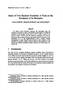
INSERT FIGURE 1 ABOUT HERE The ARL and SDRL of the two one-sided EWMA-RZ control charts can be numerically evaluated by using the formulas presented above. Without loss of generality, we assume in the remaining part of this section that z0 = 1. For the EWMA-RZ+ control chart the interval between z0 = 1 and U CL+ = K + > 1 + (see Figure 1) is divided into p subintervals of width 2δ, where δ = K 2p−1 . For the EWMA-RZ− chart the interval between z0 = 1 and LCL− = K − < 1 is − divided into p subintervals of width 2δ, where δ = 1−K 2p . By definition, each Hj , j = 1, . . . , p, represents the midpoint of the jth subinterval and H0 = z0 = 1 corresponds to the “restart state” feature of our charts (i.e. the max(. . . ) and min(. . . ) in (15) and (16), respectively). When the number p of subintervals is sufficiently large, (say p = 200), this finite approach provides an effective method that allows the run-length properties of the EWMA-RZ control charts to be accurately evaluated. In our particular case, the generic element Qi,j , i = 0, 1, . . . , p, of the matrix Q of transient probabilities is equal to • if j = 0 (for the EWMA-RZ+ chart),   1 − (1 − λ+ )Hi γ , γ , τ, ρ Qi,0 = FZˆi 1 X Y λ+

• if j = 0 (for the EWMA-RZ− chart),   1 − (1 − λ− )Hi Qi,0 = 1 − FZˆi γX , γY , τ, ρ1 λ−

(22)

(23)

• if j = 1, 2, . . . , p (for the EWMA-RZ− and EWMA-RZ+ control charts), Qi,j = FZˆi



 Hj + δ − (1 − λ)Hi γ , γ , τ, ρ 1 X Y λ   Hj − δ − (1 − λ)Hi − FZˆi γ , γ , τ, ρ (24) 1 X Y λ

where FZˆi (. . . ) is the c.d.f. of Zˆi as defined in (14) and where λ in (24) is either λ+ or λ− . Finally, concerning the zero-state condition, the vector q of initial probabilities is equal to q = (1, 0, . . . , 0). In practice, the design of the two one-sided EWMA-RZ control charts consists in selecting the optimal couples (λ−∗ , K −∗ ) or (λ+∗ , K +∗ ) which minimize 7

the out-of-control ARL for the anticipated shifts of the in-control ratio and the coefficient of correlation subject to a constraint on the in-control ARL. These optimal couples can be obtained using the following two-steps optimization procedure: 1. Find the set of design couples (λ− , K − ) or (λ+ , K + ) such that ARL = ARL0 (where ARL0 is some predefined “in-control” ARL value). 2. Choose, among these design couples (λ− , K − ) or (λ+ , K + ), the couple (λ−∗ , K −∗ ) or (λ+∗ , K +∗ ) which provides the best statistical performance, i.e. the smallest “out-of-control” ARL value for a particular shift τ in the in-control ratio z0 and for a particular shift in the coefficient of correlation from ρ = ρ0 to ρ = ρ1 . INSERT TABLE 1 ABOUT HERE

5

Numerical Analysis

The optimal couples of design parameters (λ−∗ , K −∗ ) or (λ+∗ , K +∗ ) for the two one-sided EWMA-RZ control charts have been selected by constraining the incontrol ARL at the value ARL0 = 200. For comparison purposes, the values of n, γX , γY , ρ0 , ρ1 and τ considered in this paper are the same as those investigated by Celano and Castagliola 5 i.e. n ∈ {1, 5, 15}, γX ∈ {0.01, 0.2}, γY ∈ {0.01, 0.2}, ρ0 ∈ {−0.8, −0.4, 0, 0.4, 0.8}, τ ∈ {0.90, 0.95, 0.98, 0.99, 1.01, 1.02, 1.05, 1.10} for the conditions γX = γY , γX 6= γY , ρ0 = ρ1 and ρ0 6= ρ1 . The optimal couples (λ−∗ , K −∗ ) and (λ+∗ , K +∗ ) in Table 1 correspond to the EWMA-RZ− chart when τ ∈ {0.90, 0.95, 0.98, 0.99} and correspond to the EWMA-RZ+ chart when τ ∈ {1.01, 1.02, 1.05, 1.10}. For computational reasons, (i.e. convergence of the Markov chain method), the optimal values for λ+ and λ− are always kept larger than 0.05. For the sake of brevity, Table 1 only presents the optimal design parameters for the condition γX = γY . A similar table for γX 6= γY is not presented here but is available upon request from authors. Some simple conclusions can be drawn from Table 1 • When ∆τ =|τ − 1| increases, the values of λ−∗ and λ+∗ increase to 1. For example, when (γX , γY ) = (0.01, 0.01), ρ0 = ρ1 = −0.8 and n = 15 we have λ− = 0.5153(1.0000) if τ = 0.99(0.90), i.e. ∆τ = 0.01(0.1) and we have λ+ = 0.0764(1.0000) if τ = 1.01(1.10), i.e. ∆τ = 0.01(0.1). Futhermore, the values of K − decrease and the values of K + increase as ∆τ increases. For example, when (γX , γY ) = (0.2, 0.2), ρ0 = ρ1 = −0.8 and n = 15 we have K − = 0.9696(0.9218) if τ = 0.99(0.90), i.e. ∆τ = 0.01(0.1) and we have K + = 1.0376(1.0823) if τ = 1.01(1.10), i.e. ∆τ = 0.01(0.1). • Given (γX , γY ), ρ0 and τ the values of λ−∗ and λ+∗ change with n and, in particular, λ−∗ and λ+∗ increase as n increases. For example, when (γX , γY ) = (0.01, 0.01) and ρ0 = ρ1 = 0.4, τ = 0.98(1.02) we have λ− = 8

0.4465 (λ+ = 0.4173) if n = 1 and we have λ− = 1.0000 (λ+ = 0.9985) if n = 15. • When γX = γY , given n, ρ0 and τ , the values of (λ−∗ , K −∗ ) and (λ+∗ , K +∗ ) depend on (γX , γY ). In particular, with smaller coefficients of variation (γX , γY ), the values of λ−∗ and λ+∗ are larger. Futhermore, the values of K − increase and the values of K + decrease when the coefficients of variation (γX , γY ) increase. For example, when n = 1, ρ0 = ρ1 = 0.4 and τ = 1.02 we have λ+ = 0.4143 and K + = 1.0149 when (γX , γY ) = (0.01, 0.01) and we have λ+ = 0.0500 and K + = 1.1063 when (γX , γY ) = (0.2, 0.2). The out-of-control ARL1 values for the Shewhart-RZ and EWMA-RZ control charts are shown in Figure 2 (for γX = γY ) and in Figure 3 (for γX 6= γY ), for n ∈ {1, 15} and when the process shifts from the in-control to the out-ofcontrol condition without any change in the correlation between X and Y , i.e. ρ0 = ρ1 = ρ. Numerical results have also been obtained for n = 5 but they are not presented here and are available upon request from authors. Given the results shown in Figures 2 and 3, the discussion can be summarized as follows, (we also comment on the SDRL values even if they are not shown in the two figures): • The performance of the one-sided EWMA-RZ control charts depends on (γX , γY ) and ρ0 . With smaller coefficients of variation (γX , γY ), the onesided EWMA-RZ control charts have significantly better performance in the detection of the out-of-control condition. For example, when ρ0 = 0.4, n = 15 and τ = 0.99, we get ARL1 = 1.2 and SDRL1 = 0.5 if (γX , γY ) = (0.01, 0.01); we get ARL1 = 63.5 and SDRL1 = 53.0 if (γX , γY ) = (0.2, 0.2). Occurrence of negative correlation (ρ0 < 0), between the random variables X and Y reduces the chart sensitivity vs. positive correlation, (ρ0 > 0). For instance, if (γX , γY ) = (0.2, 0.2), τ = 0.99, n = 15 and ρ0 = −0.4 we have ARL1 = 90.1 and SDRL1 = 79.5, compared to ARL1 = 63.5 and SDRL1 = 53.0 if ρ0 = 0.4. • For positive correlation between the random variables X and Y , n ≥ 1 and (γX , γY ) = (0.01, 0.01), the one-sided EWMA-RZ charts are very sensitive to a process shift, i.e. we have ARL1 ≃ 1 and SDRL1 ≃ 0 when τ < 0.99 or τ > 1.01, see for instance Figure 2 for n = 15. • It can be seen that, for the same absolute value of the ratio percentage variation ∆Z = 100 × ∆τ , the statistical performance of the EWMA-RZ charts is not identical. Furthermore, the performance difference depends on (γX , γY ). For example, when (γX , γY ) = (0.01, 0.01), n = 1, ρ0 = 0.4, and τ = 0.98 (1.02), i.e. ∆Z = 2% we have ARL1 = 3.1 and SDRL1 = 1.7 (ARL1 = 3.2 and SDRL1 = 1.7) for the EWMA-RZ− (EWMA-RZ+ ) chart, see Figure 2. Similarly, when (γX , γY ) = (0.01, 0.2), n = 1, ρ0 = 0.4 and τ = 0.98 (1.02), we get ARL1 = 97.0 and SDRL1 = 88.9 (ARL1 = 112.6 and SDRL1 = 96.4) for the EWMA-RZ− (EWMA-RZ+ ) chart, see Figure 3. 9

• Finally, for the same value of ∆Z , the statistical performance of EWMARZ charts is higher when τ < 1 and γX = γY . For instance, when (γX , γY ) = (0.2, 0.2), n = 1, ρ0 = 0.4 and τ = 0.98 (1.02), i.e. ∆Z = 2% we have ARL1 = 109.7 and SDRL1 = 100.2 (ARL1 = 111.2 and SDRL1 = 97.4) for the EWMA-RZ− (EWMA-RZ+ ) chart. Conversely, when γX 6= γY the trend of EWMA-RZ chart’s sensitivity depends on the smaller coefficient of variation between γX and γY . Specifically, for γX < γY , the statistical performance of EWMA-RZ charts is higher when τ < 1. In contrast, for γX > γY , the statistical performance of EWMA-RZ charts is higher when τ > 1. For example, when (γX , γY ) = (0.01, 0.2), n = 1, ρ0 = 0.4 and τ = 0.98 (1.02) we have ARL1 = 97.0 and SDRL1 = 88.9 (ARL1 = 112.6 and SDRL1 = 96.4) for the EWMA-RZ− (EWMA-RZ+ ) chart. Conversely, when (γX , γY ) = (0.2, 0.01), we get ARL1 = 103.0 and SDRL1 = 91.1 (ARL1 = 92.1 and SDRL1 = 81.1) for the EWMA-RZ− (EWMA-RZ+ ) chart. INSERT FIGURE 2 ABOUT HERE INSERT FIGURE 3 ABOUT HERE Figures 4 and 5 present the out-of-control ARL1 values of the ShewhartRZ and EWMA-RZ control charts when ρ0 6= ρ1 and, more particularly, for the in-control correlation coefficients ρ0 = ±0.4 and shifts from ρ0 to ρ1 = 0.5 × ρ0 and ρ1 = 2 × ρ0 , i.e. (ρ0 , ρ1 ) = {(−0.4, −0.2), (−0.4, −0.8), (0.4, 0.2), (0.4, 0.8)}. It is worth noting that if the assignable cause only shifts the incontrol correlation coefficient ρ0 but not the nominal ratio value z0 , then the incontrol ARL changes, that is ARL0 6= 200. Whatever the shift size, the results obtained in Figures 4 and 5 show a similar tendency as the results shown by Celano and Castagliola 5. These results can be summarized as follows: • the reduction of negative correlation deteriorates the sensitivity of the control chart. For example, when (γX , γY ) = (0.2, 0.2), n = 1, ρ1 = 0.5×ρ0 = −0.2 and τ = 0.98, we have ARL1 = 161.6 and SDRL1 = 151.8 for the EWMA-RZ− chart. If ρ1 = ρ0 = −0.4, we have ARL1 = 134.1 and SDRL1 = 125.3. The opposite occurs if the level of negative correlation increases: for instance, when ρ1 = 2 × ρ0 = −0.8 we get ARL1 = 86.5 and SDRL1 = 84.3 for the EWMA-RZ− chart. • the reduction of positive correlation enhances the sensitivity of the control chart. For example, when (γX , γY ) = (0.2, 0.01), n = 1, ρ1 = 0.5 × ρ0 = 0.2 and τ = 1.02, we have ARL1 = 109.4 and SDRL1 = 93.5 for the EWMA-RZ+ chart. If ρ1 = ρ0 = 0.4, we have ARL1 = 92.1 and SDRL1 = 81.1. The opposite occurs if the level of positive correlation increases: for instance, when ρ1 = 2 × ρ0 = 0.8 we get ARL1 = 119.6 and SDRL1 = 102.9 for the EWMA-RZ+ chart. A comparison with the ARL1 values of the Shewhart-RZ control chart obtained in Celano and Castagliola 5 shows that, in general, the EWMA-RZ control 10

charts outperform the Shewhart-RZ control chart when τ ∈ [0.9, 1) ∪ (1, 1.1], i.e for small and moderate shift sizes of the in-control ratio z0 : as expected, the EWMA-RZ control charts are more sensitive than the Shewhart-RZ chart. INSERT FIGURE 4 ABOUT HERE INSERT FIGURE 5 ABOUT HERE When the exact value of the shift size τ can be anticipated at the design stage by a quality practitioner, the EWMA-RZ charts can be optimally designed in terms of ARL (as we did up to now). In practice, however, the shift size to the out-of-control condition is not deterministic and cannot be predicted with sufficient precision. It is well known that a control chart can have a poor performance if the actual shift size during the process is different from the one used to design the control chart. For this reason, several potential statistical distributions fitting the unknown shift size have been considered in the literature. In particular, the uniform distribution has been proposed to account for the unknown shift size in several papers: see Chen and Chen 8 for the design of EWMA and CUSUM charts for uncertain shift sizes with different levels of quality impacts and Celano et al. 7 , who have studied control charts for short production runs and unknown shift sizes. The main idea is that if a quality practitioner has an interest to detect a range of shifts Ω = [a, b], but no preference for any particular size of the process shift, then a uniform distribution for the shift size τ can be considered over Ω, see Celano and Castagliola 5. Then, the optimal design solution problem consists of finding new unique optimal couples (λ−∗ , K −∗ ) or (λ+∗ , K +∗ ) which depend on the selected control chart, such that • For the EWMA-RZ− chart: (λ−∗ , K −∗ ) = argmin EARL(n, K − , λ− , γX , γY , ρ0 , ρ1 ) (λ− ,K − )

subject to the constraint ARL(n, K − , λ− , γX , γY , ρ0 , ρ1 = ρ0 , τ = 1) = ARL0 , • For the EWMA-RZ+ chart: (λ+∗ , K +∗ ) = argmin EARL(n, K + , λ+ , γX , γY , ρ0 , ρ1 ) (λ+ ,K + )

subject to the constraint ARL(n, K + , λ+ , γX , γY , ρ0 , ρ1 = ρ0 , τ = 1) = ARL0 , where EARL (Expected Average Run Length) is equal to Z EARL = ARL × fτ (τ )dτ, Ω

11

(25)

1 with fτ (τ ) = b−a for τ ∈ Ω = [a, b] and ARL is defined as in (17). Once again, we fixed ARL0 = 200. The new unique optimal couples (λ−∗ , K −∗ ) and (λ+∗ , K +∗ ) are not presented in this paper but are available upon request from authors. Tables 2 and 3 show the values of the EARL for Ω = [0.9, 1) (decreasing case, denoted as (D) in Tables 2 and 3) and Ω = (1, 1.1] (increasing case, denoted as (I) in Tables 2 and 3) for the conditions ρ0 = ρ1 and ρ0 6= ρ1 , respectively. The EARL values in Tables 2 and 3 show a similar tendency as for the deterministic shift size results discussed above. Furthermore, the results presented in Tables 2 and 3 also reveal something more:

• when γX = γY , the EWMA-RZ control charts have an approximately symmetrical performance for small values of γX and γY . For example, when (γX , γY ) = (0.01, 0.01), n = 5, ρ0 = −0.4, we get EARL = 1.5 for both the increasing and decreasing cases, see Table 2. This finding is independent of a shift in the coefficient of correlation, that is for ρ0 6= ρ1 , see Table 3. For larger values of γX and γY , the statistical sensitivity depends on the out-of-control correlation coefficient ρ1 . When ρ1 = ρ0 , the statistical sensitivity is slightly better for Ω = [0.9, 1) than for Ω = (1, 1.1]. For example, when (γX , γY ) = (0.2, 0.2), n = 5, ρ0 = ρ1 = −0.4, we get EARL = 42.7 for the decreasing case and EARL = 44.2 for the increasing case, see Table 2. When ρ1 > ρ0 the statistical sensitivity is slightly better for Ω = [0.9, 1) than for Ω = (1, 1.1]. For example, when (γX , γY ) = (0.2, 0.2), n = 5, ρ0 = 0.4, ρ1 = 0.8, we get EARL = 141.2 for the decreasing case and EARL = 186.6 for the increasing case. When ρ1 < ρ0 and n ≤ 5 the statistical sensitivity is slightly better for Ω = (1, 1.1] than for Ω = [0.9, 1). For example, when (γX , γY ) = (0.2, 0.2), n = 1, ρ0 = 0.4, ρ1 = 0.2, we get EARL = 46.4 for the decreasing case and EARL = 43.8 for the increasing case, see Table 3. • when γX 6= γY , the statistical sensitivity depends on the values of γX and γY . If γX < γY , then the statistical sensitivity is better for Ω = [0.9, 1) than for Ω = (1, 1.1]. For example, when (γX , γY ) = (0.01, 0.2), n = 5, ρ0 = ρ1 = −0.4, we get EARL = 26.1 for the decreasing case and EARL = 29.4 for the increasing case, see Table 2. The opposite situation occurs for γX > γY . For example, when (γX , γY ) = (0.2, 0.01), n = 5, ρ0 = ρ1 = −0.4, we get EARL = 27.7 for the decreasing case and EARL = 26.6 for the increasing case, see Table 2. It is interesting to note that this finding is independent of a shift in the coefficient of correlation, that is for ρ0 6= ρ1 , see Table 3. INSERT TABLE 2 ABOUT HERE INSERT TABLE 3 ABOUT HERE The performance comparison between EARL values of the EWMA-RZ control charts with the EARL values obtained in Celano and Castagliola 5 for the Shewhart-RZ control chart (see Tables VI–VII) is provided in Tables 4 and 12

5. The performance comparison has been undertaken by defining the following index ∆E ∆E = 100 ×

EARLShewhart−RZ − EARLEWMA−RZ , EARLShewhart−RZ

(26)

where EARLShewhart−RZ (EARLEWMA−RZ ) is the EARL value for the ShewhartRZ (EWMA-RZ) control chart. If ∆E > 0, then the EWMA-RZ charts outperform the Shewhart-RZ chart; if ∆E < 0, then the Shewhart-RZ chart outperforms the EWMA-RZ charts. It is important to note that ∆E (for the random shift case) must not be confounded with ∆Z (already introduced for the deterministic shift case). The obtained results presented in Tables 4 and 5 (rounded to the nearest integer) show that: • when γX = γY , the EWMA-RZ charts outperforms the Shewhart-RZ chart. In some case, the results for the EWMA-RZ charts are very similar to those of the Shewhart-RZ control chart for small values of γX and γY . For example, when ρ0 = ρ1 = 0, γX = γY = 0.01, for both the increasing and decreasing case, we get ∆E = 62 with n = 1 and ∆E = 0 with n = 15, see Table 4. For larger values of γX and γY , the EWMA-RZ charts always outperforms the Shewhart-RZ chart. For example, when ρ0 = ρ1 = 0.8, n = 15, γX = γY = 0.2 for both the increasing and decreasing cases, we get ∆E = 70, see Table 4 and Table 5. These findings still hold in presence of a shift of the coefficient of correlation, that is for ρ0 6= ρ1 , see Table 5. • when γX 6= γY , the EWMA-RZ charts always outperform the ShewhartRZ chart. For example, when ρ0 = ρ1 = 0.8, n = 15, γX = 0.01, γY = 0.2, we get ∆E = 65 for the decreasing case and ∆E = 74 for the increasing case, see Table 4. These findings also hold in presence of a shift of the coefficient of correlation, that is for ρ0 6= ρ1 , see Table 5. INSERT TABLE 4 ABOUT HERE INSERT TABLE 5 ABOUT HERE

6

Illustrative example

In this Section an EWMA-RZ control chart to monitor the same dataset presented in Celano and Castagliola 5, which simulates a real quality control problem from the food industry. A muesli brand recipe is produced by using a mixture of several ingredients including sunflower oil, wildflower honey, seeds (pumpkin, flaxseeds, sesame, poppy), coconut milk powder and rolled oats. To meet the food’s nutrient composition requirements declared in the brand packaging label and to preserve the mixture taste, the recipe calls for equal weights of “pumpkin seeds” and “flaxseeds”. Furthermore, their nominal proportions to the total weight of box content are both fixed at pp = pf = 0.1. To satisfy the needs of customers, the brand boxes are manufactured in different sizes. 13

According to Celano and Castagliola 5, whichever is the package dimension, the quality practitioner wants to perform on-line SPC monitoring at regular interµ vals i = 1, 2, . . . to check deviations from the in-control ratio z0 = µp,i = 0.1 0.1 = 1 f,i due to problems occurring at the dosing machine. Here, µp,i and µf,i are the mean weights for “pumpkin seeds” and “flaxseeds”, respectively. The quality practitioner collects a sample of n = 5 boxes every 30 minutes. Because the box size is allowed to change from one sample to another, it is possible to have µp,i 6= µp,k and µf,i 6= µf,k , ∀i 6= k. In the quality control laboratory, a mechanical procedure separates the “pumpkin seeds” and “flaxseeds” fromPthe muesli ¯ p,i = 1 n Wp,i,j mixture filling each box and the sample average weights W j=1 n ¯ p,i ¯ f,i = 1 Pn Wf,i,j are recorded. Finally, the ratio Zˆi = W is comand W ¯ n

j=1

Wf,i

puted and plotted on the EWMA-RZ control chart. For this example, like in Celano and Castagliola 5 , for i = 1, 2, . . . , and j = 1, 2, . . . , n both Wp,i,j and Wf,i,j can be well approximated as normal variables with constant coefficients of variation γp = 0.02 and γf = 0.01, i.e. Wp,i,j ∼ N (µp,i , 0.02 × µp,i ) and Wf,i,j ∼ N (µf,i , 0.01 × µf,i ). Moreover, the in-control correlation coefficient between these two variables is ρ0 = 0.8. In practice, accordingly to the process engineer experience, a shift of 1% in the ratio should be interpreted as a signal that something is going wrong in the production of the muesli boxes, see Celano and Castagliola 5. For this reason, the quality practitioner fixes the anticipated shift size of the ratio at τ = 1.01 and decides to implement an EWMA-RZ+ control chart. INSERT TABLE 6 ABOUT HERE INSERT FIGURE 6 ABOUT HERE For n = 5, ρ0 = 0.8, τ = 1.01, the optimal chart parameters for the EWMARZ+ chart are λ+ = 0.3938 and K + = 1.007754, i.e. U CL+ = 1.007754 × 1 = 1.007754. Table 6 shows the set of simulated sample data collected from the process (based on Celano and Castagliola 5 ), the corresponding box sizes 250– 500 gr, the Zˆi and Yi+ statistics. The process is assumed to run in-control up to sample #10. Then, between samples #10 and #11, Celano and Castagliola 5 have simulated the occurrence of an assignable cause shifting z0 = 1 to z1 = 1.01 × z0 , i.e. a ratio percentage increase equal to 1%. Figure 6 shows the EWMA-RZ+ control chart, which signals the occurrence of the out-of-control condition by plotting point #12 above the control limit U CL+ = 1.007754 (see also bold values in Table 6). The process is allowed to continue, while corrective actions are started by the repair crew who find and eliminate the assignable cause after sample #15 and restore the process back to the in-control condition.

7

Conclusions

In this paper we presented two separate one-sided EWMA control charts to monitor the ratio Z = X Y of two normal variables when subgroups of n > 1 14

sample units are collected. The size of each sample unit is allowed to change from one subgroup to another. The evaluation of the statistical performance of the proposed EWMA control charts is based on a Markov chain methodology as well as on an efficient normal approximation of the distribution of Z. For different values of the in-control coefficients of variation (γX , γY ) and correlation coefficient ρ, we have generated tables and figures presenting the optimal out-of-control ARL1 values. If the process shifts from the in-control ratio z0 to the out-of-control condition z1 = τ × z0 without a change in the in-control correlation coefficient ρ0 between X and Y , the main conclusions that can be drawn from our results are: a) with smaller coefficients of variation (γX , γY ), the one-sided EWMA-RZ control charts have a significantly better performance in the detection of the out-of-control condition than the Shewhart-RZ control chart, and the presence of negative correlation, (ρ0 < 0), between the random variables X and Y reduces the chart sensitivity vs. positive correlation, b) For the same absolute value of the ratio percentage variation ∆Z = 100 × |τ − 1|, the statistical performance of EWMA-RZ charts is not identical, c) A comparison with the performance of the Shewhart-RZ control chart shows that the proposed EWMA-RZ control charts always have a better statistical sensitivity when τ ∈ [0.99, 1) ∪ (1, 1.01]. When the occurrence of an out-of control condition is assumed to shift the in-control ratio z0 to z1 = τ × z0 as well as the in-control correlation coefficient ρ0 to ρ1 , some more conclusions can be drawn: d) the reduction of negative correlation deteriorates the sensitivity of the control chart, the opposite occurs if the level of negative correlation increases, e) the reduction of positive correlation enhances the sensitivity of the control chart. Because in industrial situations the true value of the shift size cannot be anticipated and its distribution is never known a priori, we also advocate for the use of the expected value of the out-of-control ARL, (i.e. the EARL), computed for an uniform distribution of the shift size. The main conclusions that can be drawn are: f) when γX = γY , the EWMA-RZ control charts have an approximately symmetrical performance for small values of γX and γY . In this case, for larger values of γX and γY , the statistical sensitivity depends on the out-of-control correlation coefficient ρ1 , g) when γX 6= γY the statistical sensitivity depends on the values of γX and γY , h) a comparison with the EARL values obtained in Celano and Castagliola 5 for the Shewhart-RZ control chart shows the statistical outperformance of the EWMA-RZ control charts. Future research about control charts monitoring the ratio of random normal variables should be focused on the investigation of their Phase I implementation, on the extension to CUSUM type charts, on studying the effect of the parameters estimation and the presence of measurement errors on the control charts statistical properties.

15

References [1] Ali, M., Pal, M. and Woo, J. 2007, ‘On the Ratio of Inverted Gamma Variates’, Austrian Journal of Statistics 36(2), 153–159. [2] Brook, D. and Evans, D. 1972, ‘An Approach to the Probability Distribution of CUSUM Run Length’, Biometrika 59(3), 539–549. [3] Castagliola, P. 2005, ‘A New S 2 -EWMA Control Chart for Monitoring the Process Variance’, Quality and Reliability Engineering International 21(8), 781–794. [4] Castagliola, P., Celano, G. and Psarakis, S. 2011, ‘Monitoring the Coefficient of Variation using EWMA Charts’, Journal of Quality Technology 43(3), 249–265. [5] Celano, G. and Castagliola, P. 2014, ‘Design of a Phase II Control Chart for Monitoring the Ratio of two Normal Variables’, Quality and Reliability Engineering International . DOI:10.1002/qre.1748, In press. [6] Celano, G., Castagliola, P., Faraz, A. and Fichera, S. 2014, ‘Statistical Performance of a Control Chart for Individual Observations Monitoring the Ratio of two Normal Variables’, Quality and Reliability Engineering International 30(8), 1361– 1377. [7] Celano, G., Castagliola, P., Nenes, G. and Fichera, S. 2013, ‘Performance of t Control Charts in Short Runs with Unknown Shift Sizes’, Computers & Industrial Engineering 64, 56–68. [8] Chen, A. and Chen, Y. K. 2007, ‘Design of EWMA and CUSUM Control Charts Subject to Random Shift Sizes and Quality Impacts’, IIE Transactions 39(12), 1127–1141. [9] Crowder, S. 1987, ‘A Simple Method for Studying Run-Length Distributions of Exponentially Weighted Moving Average Charts’, Technometrics 29(4), 401–407. [10] Davis, R. and Woodall, W. 1991, Evaluation of Control Charts for Ratios, in ‘22nd Annual Pittsburgh Conference on Modeling and Simulation’, Pittsburgh, PA. [11] Geary, R. 1930, ‘The Frequency Distribution of the Quotient of Two Normal Variates’, Journal of the Royal Statistical Society 93(3), 442–446. [12] Hayya, J., Armstrong, D. and Gressis, N. 1975, ‘A Note on the Ratio of Two Normally Distributed Variables’, Management Science 21(11), 1338–1341. [13] Hunter, J. 1986, ‘The Exponentially Weighted Moving Average’, Journal of Quality Technology 18, 203–210. [14] Latouche, G. and Ramaswami, V. 1999, Introduction to Matrix Analytic Methods in Stochastic Modelling, Series on Statistics and Applied Probability. SIAM, Philadelphia, PA. [15] Lucas, J. and Saccucci, M. 1990, ‘Exponentially Weighted Moving Average Control Schemes: Properties and Enhancements’, Technometrics 32(1), 1–12. [16] Montgomery, D. 2009, Statistical Quality Control: a Modern Introduction, Wiley, New York. [17] Neuts, M. 1981, Matrix-Geometric Solutions in Stochastic Models: an Algorithmic Approach, Dover Publications Inc, Baltimore, MD. ¨ ΩOksoy et al. ¨ [18] Oksoy, D., Boulos, E. and Pye, L. 1994, ‘Statistical Process Control by the Quotient of two Correlated Normal Variables’, Quality Engineering 6(2), 179–194.

16

[19] Roberts, S. 1959, ‘Control Chart Tests Based on Geometric Moving Averages’, Technometrics 1(3), 239–250. [20] Robinson, P. and Ho, T. 1978, ‘Average Run Lengths of Geometric Moving Average Charts by Numerical Methods’, Technometrics 20(1), 85–93. [21] Shu, L., Jiang, W. and Wu, S. 2007, ‘A One-Sided EWMA Control Chart for Monitoring Process Means’, Communications in Statistics – Simulation and Computation 36(4), 901–920. [22] Spisak, A. 1990, ‘A Control Chart for Ratios’, Journal of Quality Technology 22(1), 34–37. [23] Tran, K. P., Castagliola, P. and Celano, G. 2015, ‘Monitoring the Ratio of two Normal Variables using Run Rules Type Control Charts’, International Journal of Production Research . DOI:10.1080/00207543.2015.1047982, In press.

17

U CL+ = K + Hp

2δ

Hi+1 Hi Hi−1

H1

z0 = H 0 = 1

Figure 1: EWMA-RZ+ control chart. Discretization of the interval between z0 = 1 and U CL+ = K + into p subintervals of width 2δ.

18

(γX = 0.01, γY = 0.01) n=5

(γX = 0.2, γY = 0.2) n=5

n = 15

(0.0847, 0.9288) (0.0500, 0.9507) (0.0500, 0.9507) (0.0500, 0.9507) (0.0500, 1.0714) (0.0500, 1.0714) (0.0500, 1.0714) (0.0843, 1.0993)

(0.2102, 0.9218) (0.0688, 0.9621) (0.0500, 0.9696) (0.0500, 0.9696) (0.0500, 1.0376) (0.0500, 1.0376) (0.0733, 1.0482) (0.1701, 1.0823)

ρ0 = ρ1 = −0.4 (1.0000, 0.9889) (0.0500, 0.9143) (1.0000, 0.9889) (0.0500, 0.9143) (0.9995, 0.9889) (0.0500, 0.9143) (0.6242, 0.9924) (0.0500, 0.9143) (0.6086, 1.0076) (0.0500, 1.1880) (1.0000, 1.0112) (0.0500, 1.1880) (1.0000, 1.0112) (0.0500, 1.1880) (1.0000, 1.0112) (0.0500, 1.1880)

(0.1062, 0.9256) (0.0500, 0.9557) (0.0500, 0.9557) (0.0500, 0.9557) (0.0500, 1.0615) (0.0500, 1.0615) (0.0500, 1.0615) (0.0969, 1.0937)

(0.2531, 0.9218) (0.0831, 0.9616) (0.0500, 0.9729) (0.0500, 0.9729) (0.0500, 1.0327) (0.0500, 1.0327) (0.0849, 1.0461) (0.2004, 1.0797)

(1.0000, 0.9838) (0.9999, 0.9838) (0.9201, 0.9849) (0.3605, 0.9923) (0.3478, 1.0076) (0.8993, 1.0150) (0.9999, 1.0164) (1.0000, 1.0104)

ρ0 = ρ1 (1.0000, 0.9906) (1.0000, 0.9906) (0.9999, 0.9906) (0.7762, 0.9924) (0.7592, 1.0076) (0.9999, 1.0094) (1.0000, 1.0095) (1.0000, 1.0095)

= 0.0 (0.0500, 0.9239) (0.0500, 0.9239) (0.0500, 0.9239) (0.0500, 0.9239) (0.0500, 1.1488) (0.0500, 1.1488) (0.0500, 1.1488) (0.0500, 1.1488)

(0.1392, 0.9235) (0.0500, 0.9616) (0.0500, 0.9617) (0.0500, 0.9616) (0.0500, 1.0506) (0.0500, 1.0506) (0.0545, 1.0536) (0.1179, 1.0876)

(0.3178, 0.9228) (0.1088, 0.9607) (0.0500, 0.9768) (0.0500, 0.9768) (0.0500, 1.0273) (0.0500, 1.0273) (0.1040, 1.0438) (0.2534, 1.0772)

(1.0000, 0.9722) (0.9999, 0.9722) (0.4465, 0.9847) (0.1643, 0.9919) (0.1584, 1.0081) (0.4173, 1.0149) (0.9999, 1.0286) (0.9999, 1.0286)

(1.0000, 0.9875) (1.0000, 0.9875) (0.9999, 0.9875) (0.5109, 0.9925) (0.5075, 1.0076) (0.9999, 1.0127) (1.0000, 1.0127) (1.0000, 1.0127)

ρ0 = ρ1 (1.0000, 0.9927) (1.0000, 0.9927) (1.0000, 0.9927) (0.9992, 0.9927) (0.9934, 1.0073) (0.9985, 1.0073) (1.0000, 1.0073) (1.0000, 1.0073)

= 0.4 (0.0500, 0.9371) (0.0500, 0.9371) (0.0500, 0.9371) (0.0500, 0.9371) (0.0500, 1.1063) (0.0500, 1.1063) (0.0500, 1.1063) (0.0540, 1.1115)

(0.2040, 0.9226) (0.0661, 0.9628) (0.0658, 0.9629) (0.0658, 0.9629) (0.0500, 1.0380) (0.0500, 1.0380) (0.0699, 1.0472) (0.1638, 1.0813)

(0.4566, 0.9234) (0.1600, 0.9605) (0.0501, 0.9817) (0.0500, 0.9817) (0.0500, 1.0207) (0.0500, 1.0207) (0.1465, 1.0415) (0.3632, 1.0744)

(1.0000, 0.9838) (1.0000, 0.9838) (0.9157, 0.9850) (0.3527, 0.9924) (0.3488, 1.0076) (0.8994, 1.0150) (1.0000, 1.0164) (1.0000, 1.0164)

(1.0000, 0.9927) (1.0000, 0.9927) (1.0000, 0.9927) (0.9997, 0.9927) (0.9953, 1.0073) (0.9995, 1.0073) (1.0000, 1.0073) (1.0000, 1.0073)

ρ0 = ρ1 (1.0000, 0.9958) (1.0000, 0.9958) (1.0000, 0.9958) (0.9999, 0.9958) (1.0000, 1.0042) (1.0000, 1.0042) (1.0000, 1.0042) (1.0000, 1.0042)

= 0.8 (0.1145, 0.9291) (0.0500, 0.9599) (0.0500, 0.9599) (0.0500, 0.9599) (0.0500, 1.0545) (0.0500, 1.0545) (0.0500, 1.0545) (0.0937, 1.0820)

(0.4348, 0.9248) (0.1562, 0.9608) (0.0500, 0.9815) (0.0500, 0.9815) (0.0500, 1.0209) (0.0500, 1.0209) (0.1413, 1.0410) (0.3452, 1.0730)

(0.9250, 0.9238) (0.3485, 0.9619) (0.0916, 0.9837) (0.0501, 0.9891) (0.0500, 1.0116) (0.0905, 1.0172) (0.3089, 1.0377) (0.8049, 1.0740)

τ

n=1

0.90 0.95 0.98 0.99 1.01 1.02 1.05 1.10

(0.9999, 0.9523) (0.7598, 0.9618) (0.2053, 0.9840) (0.0743, 0.9917) (0.0764, 1.0088) (0.1927, 1.0159) (0.6980, 1.0375) (1.0000, 1.0501)

(1.0000, 0.9784) (0.9999, 0.9784) (0.6399, 0.9848) (0.2414, 0.9920) (0.2320, 1.0079) (0.6125, 1.0150) (0.9998, 1.0221) (1.0000, 1.0221)

n = 15 n=1 ρ0 = ρ1 = −0.8 (1.0000, 0.9875) (0.0500, 0.9068) (1.0000, 0.9875) (0.0500, 0.9068) (1.0000, 0.9875) (0.0500, 0.9068) (0.5153, 0.9924) (0.0500, 0.9068) (0.5061, 1.0076) (0.0500, 1.2253) (0.9998, 1.0127) (0.0500, 1.2253) (1.0000, 1.0127) (0.0500, 1.2253) (1.0000, 1.0127) (0.0500, 1.2253)

0.90 0.95 0.98 0.99 1.01 1.02 1.05 1.10

(1.0000, 0.9578) (0.8789, 0.9621) (0.2429, 0.9843) (0.0885, 0.9917) (0.0874, 1.0085) (0.2316, 1.0157) (0.8176, 1.0373) (1.0000, 1.0441)

(1.0000, 0.9809) (0.9999, 0.9809) (0.7569, 0.9848) (0.2819, 0.9922) (0.2771, 1.0078) (0.7238, 1.0150) (1.0000, 1.0195) (1.0000, 1.0195)

0.90 0.95 0.98 0.99 1.01 1.02 1.05 1.10

(1.0000, 0.9642) (1.0000, 0.9642) (0.3091, 0.9845) (0.1120, 0.9919) (0.1148, 1.0085) (0.2971, 1.0155) (0.9934, 1.0369) (1.0000, 1.0371)

0.90 0.95 0.98 0.99 1.01 1.02 1.05 1.10 0.90 0.95 0.98 0.99 1.01 1.02 1.05 1.10

Table 1: Values (λ−∗ , K −∗ ) when τ ∈ {0.90, 0.95, 0.98, 0.99} and (λ+∗ , K +∗ ) when τ ∈ {1.01, 1.02, 1.05, 1.10} of the EWMA-RZ charts for γX ∈ {0.01, 0.2}, γY ∈ {0.01, 0.2}, γX = γY , ρ0 ∈ { −0.8, −0.4, 0, 0.4, 0.8}, ρ0 = ρ1 , n ∈ {1, 5, 15} and ARL0 = 200

19

(γX = 0.01, γY = 0.01) ARL 90 80 70 60 50 40 30 20 10 0 0.9

ARL 80 70 60 50 40 30 20 10 0 0.9

n=1

(γX = 0.2, γY = 0.2)

n=15

ARL 5

ρ0 = ρ1 = −0.8 ARL 200

4 3 2

150

100

100

50

50

0.95

1 τ

1.05

n=1

0.95

1 τ

n=15

ARL 5

1.05

0 1.1 0.9

ρ0 = ρ1 = −0.4 ARL 200

4 3 2

1 τ

1.05

0 1.1 0.9

0.95

1 τ

1.05

1 τ

1.05

n=1

1.1

0 0.9

150

100

100

50

50

1.1

0 0.9

0.95

1 τ

0.95

1.05

1.1

0 0.9

1 τ

1.05

1.1

1.05

1.1

1.05

1.1

1.05

1.1

1.05

1.1

n=15

ARL 200

150

1 0.95

0.95

n=15

ARL 200

150

1 0 1.1 0.9

n=1

0.95

1 τ

ρ0 = ρ1 = 0 ARL 60 50 40 30 20 10 0 0.9

n=1

n=15

ARL 5 4 3 2

1 τ

1.05

0 1.1 0.9

0.95

1 τ

1.05

150

100

100

50

50

1.1

0 0.9

0.95

1 τ

n=15

ARL 200

150

1 0.95

n=1

ARL 200

1.05

1.1

0 0.9

0.95

1 τ

ρ0 = ρ1 = 0.4 ARL 35 30 25 20 15 10 5 0 0.9

n=1

n=15

ARL 5 4 3 2 1

0.95

1 τ

1.05

0 1.1 0.9

0.95

1 τ

n=1

ARL 200

1.05

150

150

100

100

50

50

0 1.1 0.9

0.95

1 τ

n=15

ARL 200

1.05

1.1

0 0.9

0.95

1 τ

ρ0 = ρ1 = 0.8 ARL 10 9 8 7 6 5 4 3 2 1 0.9

n=1

0.95

1 τ

1.05

ARL 1.9 1.8 1.7 1.6 1.5 1.4 1.3 1.2 1.1 1 1.1 0.9

n=15

0.95

1 τ

n=1

ARL 200

1.05

150

150

100

100

50

50

0 1.1 0.9

0.95

1 τ

n=15

ARL 200

1.05

1.1

0 0.9

0.95

Figure 2: ARL1 values of the EWMA-RZ (--) and RZ (-∗-) charts for γX ∈ {0.01, 0.2}, γY ∈ {0.01, 0.2}, γX = γY20 , ρ0 ∈ {−0.8, −0.4, 0, 0.4, 0.8}, ρ0 = ρ1 , τ ∈ {0.90, 0.95, 0.98, 0.99, 1.01, 1.02, 1.05, 1.10}, n ∈ {1, 15} and ARL0 = 200

1 τ

(γX = 0.01, γY = 0.2) n=1

ARL 250

(γX = 0.2, γY = 0.01) n=15

ARL 250

ρ0 = ρ1 = −0.8 ARL 250

n=1

200

200

200

200

150

150

150

150

100

100

100

100

50

50

50

50

0 0.9

0.95

1 τ

1.05

n=1

ARL 250

0 1.1 0.9

0.95

1 τ

n=15

ARL 250

1.05

0 1.1 0.9

0.95

ρ0 = ρ1 = −0.4 ARL 250

1 τ

1.05

n=1

1.1

0 0.9

200

200

200

150

150

150

150

100

100

100

100

50

50

50

50

0.95

1 τ

1.05

0 1.1 0.9

0.95

1 τ

1.05

0 1.1 0.9

0.95

1 τ

0.95

1.05

1.1

0 0.9

1 τ

1.05

1.1

1.05

1.1

1.05

1.1

1.05

1.1

1.05

1.1

n=15

ARL 250

200

0 0.9

n=15

ARL 250

0.95

1 τ

ρ0 = ρ1 = 0 n=1

ARL 250

n=15

ARL 250

n=1

ARL 250

200

200

200

200

150

150

150

150

100

100

100

100

50

50

50

50

0 0.9

0.95

1 τ

1.05

0 1.1 0.9

0.95

1 τ

1.05

0 1.1 0.9

0.95

1 τ

n=15

ARL 250

1.05

1.1

0 0.9

0.95

1 τ

ρ0 = ρ1 = 0.4 n=1

ARL 250

n=15

ARL 250

n=1

ARL 250

200

200

200

200

150

150

150

150

100

100

100

100

50

50

50

50

0 0.9

0.95

1 τ

1.05

0 1.1 0.9

0.95

1 τ

1.05

0 1.1 0.9

0.95

1 τ

n=15

ARL 250

1.05

1.1

0 0.9

0.95

1 τ

ρ0 = ρ1 = 0.8 n=1

ARL 250

n=15

ARL 250

n=1

ARL 250

200

200

200

200

150

150

150

150

100

100

100

100

50

50

50

50

0 0.9

0.95

1 τ

1.05

0 1.1 0.9

0.95

1 τ

1.05

0 1.1 0.9

0.95

1 τ

n=15

ARL 250

1.05

1.1

0 0.9

0.95

Figure 3: ARL1 values of the EWMA-RZ (--) and Shewhart-RZ (-∗-) charts for γX ∈ {0.01, 0.2}, γY ∈ {0.01, 0.2}, γX 21 6= γY , ρ0 ∈ {−0.8, −0.4, 0, 0.4, 0.8}, ρ0 = ρ1 , τ ∈ {0.90, 0.95, 0.98, 0.99, 1.01, 1.02, 1.05, 1.10}, n ∈ {1, 15} and ARL0 = 200

1 τ

(γX = 0.01, γY = 0.01) ARL 450 400 350 300 250 200 150 100 50 0 0.9

ARL 90 80 70 60 50 40 30 20 10 0 0.9

n=1

0.95

1 τ

1.05

n=1

0.95

1 τ

1.05

ARL 450 400 350 300 250 200 150 100 50 0 1.1 0.9

ARL 90 80 70 60 50 40 30 20 10 0 1.1 0.9

(γX = 0.2, γY = 0.2)

n=15

0.95

1 τ

n=15

0.95

ρ0 = −0.4,ρ1 = −0.2

1.05

ARL 450 400 350 300 250 200 150 100 50 0 1.1 0.9

0.95

ρ0 = −0.4,ρ1 = −0.8

1 τ

1.05

ARL 100 90 80 70 60 50 40 30 1.1 0.9

0.95

n=1

1 τ

1.05

ARL 450 400 350 300 250 200 150 100 50 0 1.1 0.9

1.05

ARL 90 80 70 60 50 40 30 20 10 0 1.1 0.9

1.05

ARL 80 70 60 50 40 30 20 10 0 1.1 0.9

1.05

ARL 6.0e+005 5.0e+005 4.0e+005 3.0e+005 2.0e+005 1.0e+005 0.0e+000 1.1 0.9

n=1

1 τ

n=15

0.95

1 τ

1.05

1.1

1.05

1.1

1.05

1.1

n=15

0.95

1 τ

ρ0 = 0.4,ρ1 = 0.2 ARL 80 70 60 50 40 30 20 10 0 0.9

n=1

0.95

1 τ

1.05

ARL 80 70 60 50 40 30 20 10 0 1.1 0.9

n=15

0.95

1 τ

1.05

ARL 100 90 80 70 60 50 40 30 20 1.1 0.9

n=1

0.95

1 τ

n=15

0.95

1 τ

ρ0 = 0.4,ρ1 = 0.8 ARL 9.0e+005 8.0e+005 7.0e+005 6.0e+005 5.0e+005 4.0e+005 3.0e+005 2.0e+005 1.0e+005 0.0e+000 0.9

n=1

0.95

1 τ

1.05

ARL 9.0e+005 8.0e+005 7.0e+005 6.0e+005 5.0e+005 4.0e+005 3.0e+005 2.0e+005 1.0e+005 0.0e+000 1.1 0.9

n=15

0.95

1 τ

1.05

ARL 6.0e+005 5.0e+005 4.0e+005 3.0e+005 2.0e+005 1.0e+005 0.0e+000 1.1 0.9

n=1

0.95

1 τ

Figure 4: ARL1 values of the EWMA-RZ (--) and Shewhart-RZ (-∗-) charts for γX ∈ {0.01, 0.2}, γY ∈ {0.01, 0.2}, γX = γY , (ρ0 , ρ1 ) = {(−0.4, −0.2), (−0.4, −0.8), (0.4, 0.2), (0.4, 0.8)}, τ ∈ {0.90, 0.95, 0.98, 0.99, 1.01, 1.02, 1.05, 1.10}, n ∈ {1, 15} and ARL0 = 200

22

n=15

0.95

1 τ

1.05

1.1

(γX = 0.01, γY = 0.2) ARL 300 250 200 150 100 50 0 0.9

n=1

0.95

1 τ

1.05

n=1

ARL

ARL 300 250 200 150 100 50 0 1.1 0.9

(γX = 0.2, γY = 0.01) n=15

0.95

1 τ

n=15

ARL

ρ0 = −0.4,ρ1 = −0.2

1.05

ARL 300 250 200 150 100 50 0 1.1 0.9

0.95

ρ0 = −0.4,ρ1 = −0.8 ARL

n=1

1 τ

1.05

ARL 300 250 200 150 100 50 0 1.1 0.9

n=1

200

200

200

150

150

150

150

100

100

100

100

50

50

50

50

0.95

1 τ

1.05

0 1.1 0.9

0.95

1 τ

1.05

0 1.1 0.9

0.95

1 τ

0.95

1.05

1.1

0 0.9

1 τ

1.05

1.1

1.05

1.1

1.05

1.1

1.05

1.1

n=15

ARL

200

0 0.9

n=15

0.95

1 τ

ρ0 = 0.4,ρ1 = 0.2 n=1

ARL 250

n=15

ARL 250

n=1

ARL 250

200

200

200

200

150

150

150

150

100

100

100

100

50

50

50

50

0 0.9

0.95

1 τ

1.05

0 1.1 0.9

1.05

ARL 300 250 200 150 100 50 0 1.1 0.9

0.95

1 τ

1.05

0 1.1 0.9

0.95

1 τ

n=15

ARL 250

0 0.9

1.05

1.1

1.05

ARL 300 250 200 150 100 50 0 1.1 0.9

0.95

1 τ

ρ0 = 0.4,ρ1 = 0.8 ARL 300 250 200 150 100 50 0 0.9

n=1

0.95

1 τ

n=15

0.95

1 τ

1.05

ARL 300 250 200 150 100 50 0 1.1 0.9

n=1

0.95

1 τ

n=15

0.95

Figure 5: ARL1 values of the EWMA-RZ (--) and Shewhart-RZ (-∗-) charts for γX ∈ {0.01, 0.2}, γY ∈ {0.01, 0.2}, γX 6= γY , (ρ0 , ρ1 ) = {(−0.4, −0.2), (−0.4, −0.8), (0.4, 0.2), (0.4, 0.8)}, τ ∈ {0.90, 0.95, 0.98, 0.99, 1.01, 1.02, 1.05, 1.10}, n ∈ {1, 15} and ARL0 = 200

23

1 τ

(D) (I)

(γX = 0.01, γY = 0.01) (γX = 0.2, γY = 0.2) n = 1 n = 5 n = 15 n = 1 n = 5 n = 15 ρ0 = ρ1 = −0.8 4.4 1.7 1.2 90.2 47.7 28.7 4.5 1.7 1.2 94.7 49.2 29.8

(D) (I)

3.7 3.8

1.5 1.5

ρ0 = ρ1 = −0.4 1.1 83.1 1.1 87.5

42.7 44.2

25.4 26.4

(D) (I)

3.0 3.1

1.4 1.4

ρ0 = ρ1 = 0 1.1 74.0 1.1 78.2

36.8 38.1

21.5 22.3

(D) (I)

2.2 2.3

1.2 1.2

ρ0 = ρ1 = 0.4 1.0 61.2 1.0 64.9

29.2 30.1

16.4 17.0

(D) (I)

1.4 1.4

1.0 1.0

ρ0 = ρ1 = 0.8 1.0 38.6 1.0 41.1

16.6 17.2

8.8 9.1

(D) (I)

(γX = 0.01, γY = 0.2) (γX = 0.2, γY = 0.01) n = 1 n = 5 n = 15 n = 1 n = 5 n = 15 ρ0 = ρ1 = −0.8 55.2 26.6 15.1 59.1 28.2 15.9 68.9 29.9 16.6 53.7 27.2 15.6

(D) (I)

54.3 68.0

26.1 29.4

ρ0 = ρ1 = −0.4 14.8 58.3 16.2 52.8

27.7 26.6

15.6 15.2

(D) (I)

53.3 67.2

25.6 28.9

ρ0 = ρ1 = 0 14.5 57.4 15.9 51.9

27.2 26.1

15.3 14.9

(D) (I)

52.4 66.3

25.1 28.4

ρ0 = ρ1 = 0.4 14.2 56.6 15.6 51.0

27.0 25.6

14.9 14.5

(D) (I)

51.4 65.4

24.5 27.8

ρ0 = ρ1 = 0.8 13.8 55.7 15.2 50.1

26.2 25.0

14.6 14.2

Table 2: EARL of the EWMA-RZ charts for γX ∈ {0.01, 0.2}, γY ∈ {0.01, 0.2}, γX = γY , ρ0 ∈ {−0.8, −0.4, 0, 0.4, 0.8}, ρ0 = ρ1 , n ∈ {1, 5, 15} and ARL0 = 200, Ω = [0.9, 1), i.e.(D)ecreasing case and Ω = [1, 1.1) i.e.(I)ncreasing case. 24

(D) (I)

(γX = 0.01, γY = 0.01) (γX = 0.2, γY = 0.2) n = 1 n = 5 n = 15 n = 1 n = 5 n = 15 ρ0 = −0.4,ρ1 = −0.2 3.9 1.5 1.1 95.4 48.2 27.8 4.0 1.6 1.1 119.8 53.1 29.7 ρ0 = −0.4,ρ1 = −0.8 1.1 62.9 34.2 1.1 56.8 32.9

(D) (I)

3.5 3.5

1.5 1.5

(D) (I)

2.1 2.2

1.2 1.2

ρ0 = 0.4,ρ1 = 0.2 1.0 46.4 1.0 43.8

22.9 22.7

13.5 13.7

(D) (I)

2.4 2.4

1.2 1.2

ρ0 = 0.4,ρ1 = 0.8 1.0 273.7 1.0 1805.2

141.2 186.6

29.7 38.6

(D) (I)

21.0 21.0

(γX = 0.01, γY = 0.2) (γX = 0.2, γY = 0.01) n = 1 n = 5 n = 15 n = 1 n = 5 n = 15 ρ0 = −0.4,ρ1 = −0.2 55.4 26.5 15.0 58.8 28.0 15.7 69.6 29.8 16.4 54.5 27.1 15.4 ρ0 = −0.4,ρ1 = −0.8 14.5 57.2 27.2 15.9 49.8 25.8

(D) (I)

52.1 65.2

25.4 28.6

15.3 14.9

(D) (I)

51.2 64.9

24.7 28.0

ρ0 = 0.4,ρ1 = 0.2 14.0 56.0 15.4 49.4

26.7 25.1

14.8 14.4

(D) (I)

54.9 69.5

25.8 29.2

ρ0 = 0.4,ρ1 = 0.8 14.5 57.7 15.9 54.6

27.7 26.5

15.2 14.9

Table 3: EARL of the EWMA-RZ for γX ∈ {0.01, 0.2}, γY ∈ {0.01, 0.2}, γX = γY , ρ0 ∈ {−0.8, −0.4, 0, 0.4, 0.8}, ρ0 6= ρ1 , n ∈ {1, 5, 15} and ARL0 = 200, Ω = [0.9, 1), i.e.(D)ecreasing case and Ω = [1, 1.1) i.e.(I)ncreasing case.

25

(D) (I)

(γX = 0.01, γY = 0.01) (γX = 0.2, γY = 0.2) n = 1 n = 5 n = 15 n = 1 n = 5 n = 15 ρ0 = ρ1 = −0.8 66 43 14 52 65 69 66 45 14 50 65 69

(D) (I)

65 65

38 40

ρ0 = ρ1 = −0.4 8 55 8 53

67 67

69 70

(D) (I)

62 62

26 26

ρ0 = ρ1 = 0 0 59 0 58

68 68

70 70

(D) (I)

55 54

14 14

ρ0 = ρ1 = 0.4 0 65 0 63

70 70

70 70

(D) (I)

26 26

0 0

ρ0 = ρ1 = 0.8 0 73 0 72

71 72

70 70

(D) (I)

(γX = 0.01, γY = 0.2) (γX = 0.2, γY = 0.01) n = 1 n = 5 n = 15 n = 1 n = 5 n = 15 ρ0 = ρ1 = −0.8 49 62 66 73 75 73 69 74 73 52 63 66

(D) (I)

49 70

62 75

ρ0 = ρ1 = −0.4 65 74 74 52

75 63

73 66

(D) (I)

49 70

62 75

ρ0 = ρ1 = 0 65 74 45 52

75 63

73 66

(D) (I)

48 71

62 75

ρ0 = ρ1 = 0.4 65 74 45 52

75 63

74 66

(D) (I)

48 71

62 75

ρ0 = ρ1 = 0.8 65 75 74 51

75 63

74 66

Table 4: ∆ for the EWMA-RZ for γX ∈ {0.01, 0.2}, γY ∈ {0.01, 0.2}, ρ0 ∈ {0.8, −0.4, 0, 0.4, 0.8}, ρ0 = ρ1 , n ∈ {1, 5, 15}, ARL0 = 200, Ω = [0.9, 1), i.e. (D)ecreasing case and Ω = [1, 1.1) i.e. (I)ncreasing case. 26

(D) (I)

(γX = 0.01, γY = 0.01) (γX = 0.2, γY = 0.2) n = 1 n = 5 n = 15 n = 1 n = 5 n = 15 ρ0 = −0.4,ρ1 = −0.2 75 46 8 68 79 81 75 45 8 60 78 81

(D) (I)

45 47

25 29

ρ0 = −0.4,ρ1 = −0.8 8 32 8 39

40 44

46 48

(D) (I)

38 37

8 8

ρ0 = 0.4,ρ1 = 0.2 0 41 0 45

44 47

45 47

(D) (I)

99 99

40 40

ρ0 = 0.4,ρ1 = 0.8 0 95 0 70

95 100

100 100

(D) (I)

(γX = 0.01, γY = 0.2) (γX = 0.2, γY = 0.01) n = 1 n = 5 n = 15 n = 1 n = 5 n = 15 ρ0 = −0.4,ρ1 = −0.2 52 64 67 75 76 75 71 76 75 50 65 68

(D) (I)

42.2 67

58 72

ρ0 = −0.4,ρ1 = −0.8 62 71 71 36

72 59

71 62

(D) (I)

45 69

59 74

ρ0 = 0.4,ρ1 = 0.2 63 73 72 49

74 61

72 64

(D) (I)

55 73

66 77

ρ0 = 0.4,ρ1 = 0.8 69 77 76 57

78 67

76 70

Table 5: ∆ for the EWMA-RZ for γX ∈ {0.01, 0.2}, γY ∈ {0.01, 0.2}, (ρ0 , ρ1 ) = {(−0.4, −0.2), (−0.4, −0.8), (0.4, 0.2), (0.4, 0.8)}, n ∈ {1, 5, 15}, ARL0 = 200, Ω = [0.9, 1), i.e. (D)ecreasing case and Ω = [1, 1.1) i.e. (I)ncreasing case.

27

25.792 25.052 25.292 24.933

24.960 25.107 24.449 24.831

¯ p,i [gr] W ¯ Wf,i [gr] 25.122 25.046 24.956 24.954

25.479 25.218 25.359 25.211

25.355 25.171 25.172 25.115

Wp,i,j [gr] Wf,i,j [gr] 24.027 24.684 24.508 24.679

250 gr

24.574 24.784

24.864 24.868

25.865 25.377

25.107 24.879

24.811 24.734

25.044 24.929

1.005

1.00240

4

250 gr

25.313 25.338

24.483 24.859

24.088 24.305

25.184 25.115

25.681 25.251

24.950 24.974

0.999

1.00106

5

250 gr

25.557 25.277

24.959 25.402

25.023 25.012

24.482 24.937

25.531 25.148

25.111 25.163

0.998

1.00000

6

250 gr

24.882 24.962

24.473 24.644

24.814 24.817

25.418 25.419

24.732 24.818

24.864 24.932

0.997

1.00000

7

500 gr

49.848 49.993

48.685 49.128

49.994 49.830

49.910 49.566

49.374 49.422

49.562 49.588

0.999

1.00000

8

500 gr

49.668 49.695

50.338 50.681

49.149 49.640

47.807 48.969

49.064 49.612

49.205 49.720

0.990

1.00000

9

500 gr

51.273 50.366

48.303 49.210

48.510 49.844

50.594 49.890

48.591 49.595

49.454 49.781

0.993

1.00000

10

500 gr

48.720 49.721

51.566 50.215

49.677 50.178

50.651 50.324

50.344 50.071

50.192 50.102

1.002

1.00079

11

500 gr

51.372 50.164

51.700 50.272

51.000 49.884

50.886 50.061

49.641 49.845

50.920 50.045

1.017

1.00717

12

500 gr

52.020 50.749

53.182 50.369

51.374 49.697

51.342 49.575

48.771 49.440

51.138 49.966

1.023

1.01340

13

500 gr

52.360 50.047

49.412 49.981

50.704 50.297

50.370 50.408

50.901 50.026

50.949 50.152

1.016

1.01443

14

500 gr

52.498 50.064

50.447 50.124

48.713 49.162

48.574 48.865

50.275 50.344

50.101 49.712

1.008

1.01190

15

250 gr

25.123 25.041

24.658 24.790

24.468 24.835

25.030 25.211

25.071 25.008

24.870 24.977

0.996

1.00564

Sample 1

Box Size 250 gr

2

250 gr

3

Table 6: The food industry example data

28

¯ p,i W Zˆi = W ¯ f,i 1.003

Yi+ 1.00118

1.003

1.00072

EWMARZ+ chart 1.014 1.012 1.01

U CL+

Yi

1.008 1.006 1.004 1.002 1 1

2

3

4

5

6

7

8

9

10

11

12

13

14

15

i

Figure 6: EWMA-RZ control charts for the food industry example

29