Monitoring Volcanic Eruptions with a Wireless Sensor Network Geoffrey Werner-Allen∗ , Jeff Johnson† , Mario Ruiz‡ , Jonathan Lees‡ , and Matt Welsh∗ ∗ Harvard
University {werner, mdw}@eecs.harvard.edu † University of New Hampshire
[email protected] ‡ University of North Carolina {mruiz, leesj}@email.unc.edu
Abstract— This paper describes our experiences using a wireless sensor network to monitor volcanic eruptions with low-frequency acoustic sensors. We developed a wireless sensor array and deployed it in July 2004 at Volc´an Tungurahua, an active volcano in central Ecuador. The network collected infrasonic (low-frequency acoustic) signals at 102 Hz, transmitting data over a 9 km wireless link to a remote base station. During the deployment, we collected over 54 hours of continuous data which included at least 9 large explosions. Nodes were time-synchronized using a separate GPS receiver, and our data was later correlated with that acquired at a nearby wired sensor array. In addition to continuous sampling, we have developed a distributed event detector that automatically triggers data transmission when a well-correlated signal is received by multiple nodes. We evaluate this approach in terms of reduced energy and bandwidth usage, as well as accuracy of infrasonic signal detection.
I. I NTRODUCTION Wireless sensor networks have the potential to greatly benefit studies of volcanic activity. Volcanologists currently use wired arrays of sensors, such as seismometers and acoustic microphones, to monitor volcanic eruptions. These sensor arrays are used to determine the source mechanism and location of an earthquake or explosion, study the interior structure of the volcano, and differentiate true eruptions from noise or other signals (e.g., mining activity) not of volcanological interest. A typical campaign-type study will involve placement of one or more stations on various sites around a volcano. Each station typically consists of a few (less than five) wired sensors distributed over a relatively small area (less than 100 m2 ), and records data locally to a hard drive or flash card. The data must be manually retrieved from the station, which may be inconveniently located. Power
consumption of these systems is very high, requiring large batteries and solar panels for long deployments. Embedded wireless sensor networks, consisting of small, low-power devices integrating a modest amount of CPU, memory, and wireless communication, could play an important role in volcanic monitoring. Wireless sensor nodes have lower power requirements, are easier to deploy, and can support a larger number of sensors distributed over a wider area than current wired arrays. Using long-distance wireless links, data can be monitored in real time, avoiding the need for manual data collection from remote stations. Such an approach is not without its challenges, however. Volcanic timeseries data are often sampled continuously at rates of 40 Hz or more, far greater than the low frequencies used in environmental monitoring studies [1]. Due to limited radio bandwidth, however, complete signals cannot be captured and transmitted from a large sensor array. For such a network to run for extended periods of time, careful power management techniques, such as triggering and in-network event detection, must be developed. In addition, signals from multiple sensor nodes must be accurately synchronized against a global time base. To demonstrate the use of wireless sensors for volcanic monitoring, we developed a wireless sensor network and deployed it on Volc´an Tungurahua, an active volcano in central Ecuador. This network was based on the Mica2 sensor mote platform and consisted of three infrasonic (low-frequency acoustic) microphone nodes transmitting data to an aggregation node, which relayed the data over a 9 km wireless link to a laptop at the volcano observatory. A separate GPS receiver was used to establish a common time base for the infrasonic sensors. During this deployment, we recorded over 54 hours of infrasonic signals at a rate of 102 Hz per node, resulting
in over 1.7 GB of uncompressed log data. Throughout the deployment the volcano produced several small or moderate explosions an hour, though the rate and energy of eruptions varied considerably. This small-scale deployment provided a proof-ofconcept as well as a wealth of real acoustic signals that we have used to develop a larger-scale prototype. In order to scale to a larger number of nodes, we have developed a distributed signal correlation scheme, in which individual infrasonic motes capture signals locally and communicate only to determine whether an “interesting” event has occurred. By only transmitting well-correlated signals to the base station, radio bandwidth usage is greatly reduced. This paper describes the design, implementation, and deployment of a wireless sensor network for volcanic monitoring. This paper makes the following contributions. First, this is the first application to our knowledge of mote-based sensor arrays to volcanic studies. Second, we demonstrate that it is possible to capture infrasonic signals from an erupting volcano using a wireless sensor network, and that the captured data correlates well with a colocated, wired seismic and acoustic array. Third, we develop a distributed, in-network event detection and correlation algorithm the greatly reduces communication requirements for larger-scale sensor arrays. The rest of this paper is organized as follows. In Section II we present the scientific background for the use of infrasonic arrays to monitor volcanic activity. Section III presents the design of our wireless sensor network for capturing continuous infrasonic signals, and Section IV describes our experience with a real sensor network deployment at Volc´an Tungurahua. In Section V we describe the distributed event correlation scheme, and we evaluate its performance with respect to scalability, bandwidth, and power consumption in Section VI. Finally, Section VII presents future work and concludes. II. BACKGROUND Networks of spatially-distributed sensors are commonly used to monitor volcanic activity, both for hazard monitoring and scientific research [2]. Typical sensing instruments include seismic, acoustic, GPS, tilt-meter, optical thermal, and gas flux. Unfortunately, the number of deployed sensors at a given volcano has traditionally been limited by a variety of factors, including monetary expenses such as sensor, communication, and power costs; logistical concerns related to time and access issues; and archival and telemetry bandwidth constraints.
A. Volcanic monitoring arrays and networks Volcanic sensors range from widely dispersed instrument networks to more confined sensor arrays. An individual sensor station may consist of a single sensor (e.g., seismometer or tilt sensor), or an array of several closelyspaced (102 to 103 m aperture) wired sensors, perhaps of different types. Multiple stations may be integrated into a larger network that is installed over an extended azimuthal distribution and radial distance (102 to 104 m) from the vent. Data from the various stations may be either recorded continuously or as triggered events and the acquisition bandwidth depends upon the specific data stream. For instance, seismic data is often acquired at 24bit resolution at 100 Hz, while tilt data may be recorded with 12-bit resolution at 1 Hz or less. Sensor data at a station may be recorded locally or transmitted over long-distance radio or telephone links to an observatory located tens of kilometers from the volcano. At the receiving site, data is displayed on revolving paper helicorders for rapid general interpretation and simultaneously digitized for further processing. However, due to the expense and bandwidth constraints of radio telemetry, high-quality, multi-channel data acquisition at a particular volcano is often limited. These analog systems also suffer from signal degradation and communication interference. As a result, many scientific experiments use a standalone data acquisition system at each recording station. The digitizer performs high-resolution analog-to-digital conversion from the wired sensors and stores data on a hard drive or Compact Flash card. However, these systems are cumbersome, power hungry (≈ 10 Watts), and require data to be manually retrieved from the station prior to processing. Depending on the size of the recording media, a station may record several days or weeks’ worth of data before it must be serviced. B. Scientific and monitoring goals Volcanic monitoring has a wide range of goals, related to both scientific studies and hazard monitoring. The type and configuration of the instrumentation depends on the goals of a particular study. Traditionally, dispersed networks of seismographs, which record groundpropagating elastic energy, are utilized to locate, determine the size of, and assess focal mechanisms (source motions) of earthquakes occurring within a volcanic edifice [3]. At least four spatially-distributed seismographs are required to constrain hypocentral (3D) source location and origin time of an earthquake, though using more seismic elements enhances hypocenter resolution and
Fig. 1.
Sensor arrays for volcanic monitoring.
the understanding of source mechanisms. Understanding spatial and temporal changes in the character of volcanic earthquakes is essential for tracking volcanic activity, as well as predicting eruptions and paroxysmal events [4]. Another use of seismic networks is the imaging of the internal structure of a volcano through tomographic inversion. Earthquakes recorded by spatially-distributed seismometers provide information about propagation velocities between a particular source and receiver. A seismically-active volcano thus allows for threedimensional imaging of the volcano’s velocity structure [5], [6]. The velocity structure can then be related to material properties of the volcano, which may be used to determine the existence of a magma chamber [7], [8]. Dense array configurations, with as many as several dozen seismographs, are also an important focus of volcanic research [9], [10]. Correlated seismic body and surface wave phases can be tracked as they cross the array elements, enabling particle motion and wavefield analysis, source back-azimuth calculations, and enhanced signal-to-noise recovery. C. The role of infrasound Infrasonic signals are becoming an increasingly important means by which to study volcanic activity. An acoustic antenna, with three or more microphones that
record low-frequency sound pressure waves, are used for enhancing signal-to-noise and discriminating the source of a volcanic event [11]. In cases where the volcanic vent may not be visible due to terrain or cloud cover, infrasonic signals can help differentiate eruptive activity from other sources of seismic signals such as mining operations or bovine ambulation. In volcanoes with multiple vents, such as Stromboli, Italy, an array of acoustic sensors can triangulate the precise location of individual eruptions [12]. Combining seismic and acoustic signals in a sensor array has great potential for assessing eruption intensity and interpreting trends in volcanic activity [13]. Infrasonic signals have also been used to track non-stationary sources [14] and to understand the weather-dependent velocity structure of the atmosphere [15]. D. Opportunities for wireless sensor networks Wireless sensor networks present new opportunities for volcanic monitoring by offering increased scale and resolution. As mentioned above, analog radio telemetry has been used at volcanic monitoring stations for some time. More recently, spread-spectrum digital modems have been employed to transmit digital data from remote monitoring stations to an observatory. For example, at Mount Erebus, Antarctica, a five-station sensor array was
installed that transmits real-time data over a FreeWave modem [16] to a central PC that is connected to the Internet over a geosynchronous satellite link [17]. However, these approaches are still limited in terms of the number of individual channels (seismic, acoustic, etc.) that can be recorded at each station and the communication bandwidth of the long-distance radio link. The number and placement of sensors at a station is limited by power requirements, cable length, and data recording capabilities. For example, a typical data recorder supports only up to six 24-bit channels. The use of small, low-power, wireless sensor nodes can greatly benefit volcanic monitoring studies, allowing researchers to deploy large sensor arrays in a versatile fashion. A sensor array of tens of microphones or seismic elements will improve spatial resolution and resilience to wind noise and permit much more detailed analysis of received signals. Unlike a fixed data logger, wireless sensor networks are reprogrammable, allowing researchers to experiment with signal processing, compression, oversampling, and other techniques to improve the quality of the data captured. The use of wireless sensor networks in this context raises a number of new challenges. The data rates from individual sensors (≈ 100 Hz) are much higher than those in low data-rate applications, such as environmental monitoring [1], [18]. Therefore, new approaches to managing bandwidth are required, since even a small number of sensors will saturate the wireless link. Rather than sampling and transmitting data continuously, it is necessary to perform compression, correlation, or other processing of signals on the sensor nodes themselves. In addition, sensor nodes must be tightly time synchronized to allow signals from each node to be compared. III. S YSTEM D ESIGN In this section, we present a detailed description of our wireless sensor array for volcanic monitoring. Our initial experiment focused on establishing feasibility by capturing complete, high-resolution signals from a small number of wireless sensor nodes, and comparing this data to that from a colocated wired station. However, our system architecture can generalize to much larger deployments, as we describe in Section V. A. System architecture Our design consists of several components, shown in Figure 2. The first is a set of infrasound monitoring nodes, which sample low-frequency acoustic signals (up to 50 Hz). These nodes transmit their signals to an
aggregator node, which relays the signals over a longdistance wireless link to a wired base station, a laptop running various software tools to visualize, store, and analyze the real-time signals from the wireless array. To establish a common time base across the captured signals, a GPS receiver node is used, which receives a GPS time signal and relays the data to the infrasound and aggregator nodes through radio messages. The infrasound, aggregator, and GPS receiver nodes are based on the Mica2 mote, a typical wireless sensor device. It consists of a 7.3 MHz ATmega128L processor, 128KB of code memory, 4KB of data memory, and a Chipcon CC1000 radio operating at 433 MHz with a data rate of approximately 34 Kbps. The Mica2 runs a lean, component-oriented operating system, called TinyOS [19]. B. Infrasound node The infrasound monitoring node (Figure 3(a)) uses a custom sensor board1 consisting of an amplifier and filtering circuit connected to a Panasonic WM-034BY omnidirectional electret condenser microphone. These microphones have been used in other infrasonic monitoring studies [13] and have been found to have very good low frequency response, despite their small size. The sensor board has a manually configurable gain setting (from 1x to 20x) using a jumper block. Given the low dynamic range of the ADC on the Mica2 motes (10 bits), we used the highest gain setting during our deployment. Each infrasound node was programmed to sample data continuously at 102.4 Hz, allowing signals up to 51.2 Hz to be accurately.2 A set of 25 consecutive samples is packed into a 32-byte radio packet and transmitted at approximately 4 Hz. The radio packet header includes a sequence number (used to detect lost packets), the source node ID, and information on the most recent GPS timestamp (Section III-D). Upon receiving each packet, the aggregator node transmits a short acknowledgment. If the acknowledgment is not received by the source node, it will attempt retransmission up to 5 times. After some initial experimentation with this design, we noticed that the samples provided by the Mica2’s internal ADC were distorted during radio transmission. While the radio is in the process of transmitting a packet, any ADC readings taken were offset lower by several bits. Because 1
This board was designed by Pratheev Sreetharan at Harvard University. 2 Because the TinyOS timer component measures time in binary milliseconds, 102.4 Hz is the closest available value to our desired sampling frequency of 100 Hz.
Wireless infrasonic sensor nodes
GPS timebase Time sync pulse
Base station at observation post
Receiver
Long−distance wireless modem
Infrasound samples
System architecture of the infrasonic sensor array.
Fig. 2.
(a) Infrasonic monitoring node.
(b) FreeWave modem.
(c) Yagi antenna oriented towards observatory.
of the length of the radio message, preamble, and other overhead, up to 3 samples in a given packet may be affected by the transmission of the previous packet. We believe this is caused by the lack of an external, fixed voltage reference for the ADC, some issues with the Mica2 ground plane, as well as EM interference from the radio oscillator itself. However, due to the relatively high sample rate, we were unable to completely avoid sampling during radio transmissions. To correct this distortion, we utilized information from the TinyOS MAC layer, which allows an application component to be notified when a message is being transmitted through the RadioSendCoordinator.startSymbol() event. The difference between the last ADC reading before the transmission and the first reading during the transmission is measured. If this offset is below some small threshold, an offset is added to each ADC reading taken during transmission. While this is a very simple filter, it effectively corrects for the ADC distortion (Figure 4). This problem motivates the need good for crosslayer information flow in embedded systems software. The application’s ability to know exactly which ADC readings are affected by a radio transmission allows the
Sample data
Equipment used in our sensor network deployment.
Sample data
Fig. 3.
20 km
540 530 520 510 500 490 480 470 2200 560 550 540 530 520 510 500 490 2200
Unsmoothed data
2220
2240
2260 2280 2300 Sequence number
2320
2340
Smoothed data
2220
2240
2260 2280 2300 Sequence number
2320
2340
Fig. 4. Data filtering to correct for radio interference with
analog-to-digital signal conversion on the Mica2. The top figure shows an acoustic signal from a mote before filtering; the 4 Hz noise is caused by radio transmissions interfering with the ADC. The bottom figure shows a signal from a different mote with filtering enabled.
data to be corrected on the fly, rather than attempting to correct the signal distortion after the fact. However, better hardware designs are another solution: our initial testing of the Moteiv Telos motes [20] indicates that they do not exhibit this problem.
C. Aggregator node and long-distance data transmission The aggregator node receives infrasonic sample and GPS timestamp messages and acknowledges them, as described above. It relays each received message to its serial port, which is connected to a FreeWave spreadspectrum modem (Figure 3(b)) providing a reliable serial data connection over distances of 20 km or more. On the receiving end of the link, a second FreeWave modem is connected to a laptop base station running a Java program that logs the raw data to a series of files. Each file contains the raw contents of each received radio packet, consisting of infrasound samples from each sensor node as well as GPS timestamp messages (see below). The real-time data is also exported via a TCP socket (using the TinyOS serialforwarder program) to allow other programs to visualize or process the stream of samples in real time. All other data analysis was performed on the logged data files. D. GPS receiver node Because we are interested in correlating signals across multiple sensor nodes and comparing our signals to those captured at co-located wired sensor arrays, it is essential that we accurately timestamp the sensor data from each node. For this purpose, we made use of a Garmin GPS 18LVC receiver puck that provides a 1 Hz digital signal accurate to within 1 µsec of the GPS timebase, through a serial interface transmitting binary or ASCII NMEA 0183 GPS data. The GPS puck is connected to a separate Mica2 node acting as a GPS receiver, with the PPS time signal tied to an interrupt line. Our time synchronization protocol is similar in nature to RBS [21]. When the PPS interrupt from the GPS receiver is raised, the GPS receiver node records the local value of a 921.6 KHz timer. It then broadcasts a radio packet containing a sequence number, the GPS timestamp of the previous NMEA 0183 GGA sentence in HHM M SS format, and the delay (measured in ticks from the 921.6 KHz timer) between the PPS interrupt and the time that the node begins transmitting the message (that is, after MAC delay and backoff). Because every sensor node will receive this radio message at the same time, we can record the local time at each node when this message was received and use this information to cross-correlate the signals being captured by each infrasound node. The MAC delay reported by the GPS sender can be used to register this common timebase back to the true GPS time for comparison with other stations. Our initial deployment
only requires single-hop time synchronization, although this approach can be readily extended to multihop cases using a multihop time synchronization protocol [22]. E. Time regression To perform analysis of the data recorded across the sensor array, it is necessary to align the sample streams from each node to a common timebase. This step is performed offline on the data logged at the base station. Each log entry consists of a tuple of the form {moteid, packetno, sample}, where moteid is the ID of the transmitting mote, seqno is the sequence number for the corresponding radio packet, and sample is the 10-bit ADC sample data. Recall that 25 samples are contained in each radio message. If a GPS timestamp message was received by the node while collecting samples in this packet, the log entry will also contain two additional fields: the sequence number of the GPS timestamp message, and the index of the sample (0 to 24) that was being acquired when the GPS message was received. The true GPS time and transmission delay for each GPS timestamp is logged separately. We expect that the sampling rate of individual nodes may vary slightly over time, due to changes in temperature and battery voltage. In addition, our logs do not record the precise time that a GPS timestamp message arrives during the acquisition of a sample. To address these uncertainties, we apply a linear regression to the logged data stream, using the samples tagged with GPS timestamp arrivals as inputs to the regression. The output is the estimated sampling rate of each node over time, allowing individual samples to be mapped to a “true” time that the sample was acquired. The regression is applied to runs of logged samples with no more than 100 missing packets between runs, and with a maximum of 10,000 samples in each run. F. Physical packaging Clearly, leaving sensor nodes in an exposed environment requires appropriate physical packaging to protect the instruments from moisture, humidity, and sunlight. Our nodes were enclosed in watertight Pelican cases of various sizes, which are inexpensive, easy to open and close, and very effective at protecting against the elements. Weatherproof 1/4-wave whip antennas were used for each of the sensor nodes, which were attached to the outside of each Pelican case, and a small hole was drilled to thread the antenna pigtail inside the case. Silicone sealant was used to weatherproof this opening.
Tungurahua
Fig. 6.
Fig. 5.
Map showing location of Volc´an Tungurahua.
The microphones require open access to the atmosphere to measure incident pressure waves from the volcano. A small hole was drilled on the side of the infrasonic microphone node cases to allow approximately 1 m of coax cable attaching the microphone to the mote inside the case. The microphones themselves were protected with a makeshift wind- and rain-shield consisting of the top cut off of a two-liter plastic pop bottle. The microphone was placed inside the mouth of the bottle and oriented downwards to minimize moisture accumulation. ´ T UNGURAHUA IV. D EPLOYMENT AT VOLC AN To demonstrate the value of wireless sensor networks for volcanic monitoring, we deployed a small infrasonic monitoring network, using the design in the previous section, at Volc´an Tungurahua, an active volcano in central Ecuador. Our network consisted of three infrasonic monitoring nodes, continuously transmitting infrasonic signals at 102 Hz to a central aggregator node, which relayed the data over a wireless link to an observatory approximately 9 km from the monitoring station. The deployment was active from July 20–22, 2004 and collected over 54 hours of infrasonic signals. During this time, the volcano was erupting at the rate of several small or moderate explosions an hour. A. Volc´an Tungurahua Volc´an Tungurahua (78.43◦ W, 1.45◦ S) is located on the central part of the Eastern Cordillera of the Ecuadorean Andes (Figures 5 and 6). Its current cone has a steep flank (30-35◦ slopes) and a crater at the upper
Volc´an Tungurahua.
part of its northwestern flank. Ba˜nos, an important tourist destination in Ecuador with 25,000 inhabitants, is located at the foot of the volcano close to Agoyan, one of the country’s largest hydroelectric plants. Rural communities are dispersed all around the volcano’s lower flanks. Geological studies show that Volc´an Tungurahua has produced Plinian-type eruptions as well as at least two sector collapses (≈ 13,000 and 3,000 years b.p. [23]). Since colonial times (1534), five eruptive cycles have occurred: 1641–1646, 1773–1781, 1886–1888, 1916–1918, and 1999–present. Generally, these eruptions were characterized by tephra-and-ash falls covering the volcano flanks, especially the western slopes, lahars, pyroclastic flows, and lava flows running down the north, west and south-western valleys. The current eruptive period was preceded by anomalous seismicity first detected in 1993 by the local seismic network [24]. In October 1999, after a few months of increasing seismicity, Tungurahua emitted an ash column with incandescent blocks. This activity led to the evacuation of more than 16,000 residents from the surrounding areas. As of August 2004, more than 1,900 volcanic explosions have been recorded at Tungurahua by the Instituto Geof´ısico in Quito. Activity has been grouped into eight eruptive cycles. The last cycle started on May 2004 and reached its climax in June. These eruptive periods have manifested ash emissions, and vulcanian and strombolian activity. Volc´an Tungurahua is monitored by the Instituto Geof´ısico of the Escuela Politecnica Nacional (IGEPN) using a seismic network of seven short-period stations, one broadband station, two tiltmeters, five deformation control lines, acoustic flow meters, and an SO2 concentration measurement system. In November 1999,
0.16
Mote 2 Mote 3 Mote 4
0.14 Packet loss rate
a temporary microphone for recording infrasound signals was deployed in a ridge just in front of the volcano northwestern flank [11]. In addition, numerous scientific campaigns, such as ours, have deployed temporary monitoring stations on the volcano.
0.12 0.1 0.08 0.06 0.04 0.02 0
B. Deployment Our sensor network deployment was colocated with a wired seismic and infrasound station used by researchers from UNC and IGEPN. The deployment station was located via GPS at 78.46380◦ W, 1.43561◦ S at an elevation of 2889 m. As described previously, the aggregator node transmits data via a FreeWave modem to a laptop acting as a base station. The laptop was kept at the volcano observatory operated by IGEPN, which is located 9 km away from the monitoring station. The observatory is in a valley with direct line-of-sight to the monitoring station on the volcano. A pair of 9 dBi 900 MHz Yagi antennas (Figure 3(c)) were used to establish connectivity between the two FreeWave modems. The GPS receiver and FreeWave modem were powered by a 12 V car battery (smaller lead-acid batteries were used for testing but are disallowed on commercial air flights). All other nodes were powered by 2 AA batteries and operated continuously during the 54-hour deployment. The aggregator node, GPS receiver, FreeWave modem, Yagi antenna, and car battery were placed at the foot of a tree. One of the infrasonic nodes was placed about 1 m above ground in the same tree. Another node was placed 6.3 m away in a second tree, while the third node was placed 10.7 m away on a tree stump. Infrasound nodes were elevated in trees both to improve radio reception and to minimize molestation by cows grazing nearby. The terrain at this location was fairly steep with a large amount of vegetation, making it difficult to select locations further away from the aggregator node. C. Data analysis We logged over 54 hours of continuous data from the sensor network. Analyzing this raw data presented a number of challenges. Although the infrasound nodes use a retransmission scheme to improve reliability, a large number of packets are missing from the recorded dataset. On several occasions, the FreeWave modems would experience short dropouts of several seconds, causing data from all nodes to be lost. In addition, GPS timestamp messages from the GPS receiver may not have been received at the basestation, although the infrasound motes may have received the message. Finally, on a
07/21/2004 02:00 01:00:00 GMT
Mote node 2 node 3 node 4
03:00
04:00
05:00
06:00
Received pkts 19470100 19039684 19584438
07:00
08:00
Lost pkts 555696 995416 290525
09:00
10:00
11:00
07/21/2004 12:00:00 GMT
loss rate 2.77% 4.96% 1.46%
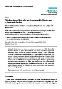
Fig. 7. Packet reception and loss statistics. The graph shows
packet loss rate, averaged over one-minute intervals, for an 11-hour trace. Mote 4 exhibited negligible losses during this time. The table summarizes packet loss over the entire 54-hour deployment.
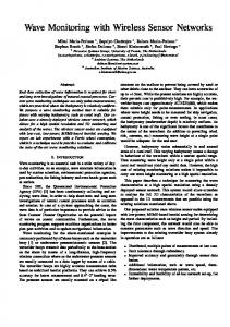
number of occasions, duplicate packets were recorded, most likely due to a lost acknowledgment and redundant retransmission. Before registering the data to a common timebase as described in Section III-E, it was necessary to “clean up” the raw logs by accounting for lost and duplicate packets. The loss rate for each node varied during the deployment. Figure 7 shows the loss rate, averaged over oneminute intervals, for an 11-hour trace. We believe that the gradual variation in loss is due to weather conditions (e.g., rain) affecting radio transmission, although it is possible that temperature fluctuations (heating and cooling of components in the Pelican cases) may have contributed to this effect as well. Mote 4 experienced very low loss, due to its positioning with a clear lineof-sight to the receiver. Note that Mote 2, despite being located in the tree above the receiver, experienced somewhat higher losses, probably due to antenna orientation. Figure 7 summarizes the packet loss rate for each of the motes during the entire deployment. Through visual inspection of the time-regressed logs, we manually verified well-correlated infrasonic signals from nine separate explosions recorded during our deployment. The frequency of explosions varied greatly, with inter-explosion times ranging from 1 hour to over 24 hours. Data recorded by our sensor array during an example explosion is shown in Figure 8. Infrasonic and seismic data from the colocated wired station is shown for comparison. As the figure shows, the wireless array demonstrates very good correlation with wired station. Note that the seismic signal precedes the acoustic by several seconds due to its faster propagation speed.
1024 0
Mote #2
126666
126668
126670
126672
126674
126676
1024
126664
126678
126680
0
Mote #3
126666
126668
126670
126672
126674
126676
1024
126664
126678
126680
0
Mote #4
126666
126668
126670
126672
126674
-0.26
126676
126678
126680
Wired infrasound
126664
126666
126668
126670
126672
126674
-0.13
0.3439
-0.9209
126664
126676
126678
126680
Wired seismic
126664
126666
126668
126670
126672
126674
126676
126678
126680
Time, sec
Example infrasonic and seismic data from an explosion at Tungurahua. The top three graphs show the signal recorded by our wireless infrasonic sensor network (July 21 2004 at 11:11:00 GMT). The bottom two graphs show infrasonic and seismic signals from the same explosion recorded by a colocated wired station.
Fig. 8.
V. D ISTRIBUTED E VENT D ETECTION Our initial deployment on Volc´an Tungurahua was small enough that it was possible to transmit continuous signals from each of the nodes. However, such an approach is not feasible for larger arrays deployed over longer periods of time. We are planning to deploy a much larger (approximately 30 node) sensor array on Tungurahua within the next 8-12 months. To save bandwidth and energy, it is desirable to avoid transmitting signals when the volcano is quiescent. In this section, we describe a distributed event detector that only transmits well-correlated signals to the base station. A. Distributed Detector Design Our distributed detector uses a decentralized voting process to measure signal correlation among a group of
nodes. Each node samples data continuously at 102.4 Hz and buffers a window of acquired data while running a local event detection algorithm. When the local event detector triggers, the node broadcasts a vote message. If any node receives enough votes from other nodes during some time window, it initiates global data collection by flooding a message to all nodes in the network. Note that in this approach, voting uses local radio broadcast, while data collection is initiated using a global flood. Our expectation is that in a typical deployment, each node will have multiple neighbors within radio range with which it can compare votes using local broadcast only. To reduce radio contention during data collection, we use a token-based scheme for scheduling transmissions. Upon initiating global data collection, the first node
B. Local Detector Design Our design decouples the distributed voting scheme from the specific local event detection algorithm used, allowing us to explore different approaches. Figure 8 shows a typical infrasonic wave. Designing a local event detector for this kind of waveform is straightforward, although some tuning is required to minimize false positives (which may trigger data collection for uncorrelated signals) and false negatives (which may cause true explosions to be missed). We have implemented two local event detectors: a threshold-based detector and an exponentially weighted moving average (EWMA)-based detector. The threshold detector is triggered whenever a signal rises above one threshold, Thi , and falls below another, Tlo , during some time window W . Because this detector relies on absolute thresholds, it is sensitive to the particular microphone gain on each node. It is also susceptible to false triggering due to spurious signals, such as wind noise, although the voting scheme described above mitigates this effect. The EWMA detector calculates two moving averages with different gain parameters, αshort and αlong , representing both short-term and long-term averages of the signal. For each ADC sample, each moving average is calculated as:
Distributed Detector Per Mote Bandwidth 45 Node 1 Node 2 Node 3 Node 4 Node 5 Node 6 Node 7 Node 8
40 35
Data transfer
30 Packets/sec
(ordered by node ID) transmits its complete buffer of data to the base station, performing retransmissions for any lost packets. Once the complete buffer has been transmitted, the node broadcasts a message indicating that the next node in the numeric sequence should transmit its buffer. If a node does not hear the token exchange (or has failed), the base station will flood the network with a data request after a timeout period, ensuring forward progress.
25 20 15 10 5 Voting 0 0
5
10
15
20
25
Time (sec)
Fig. 9. Distributed detector network bandwidth consump-
tion. Values are shown as packets per second. The voting and round-robin data collection phases are clearly visible.
our lab. The infrasonic signals used to trigger the array were produced by decisively closing the lab door, which closely mimics infrasonic signals produced by a volcano. Since the lab experiments were not intended to evaluate the accuracy of the local detector we exploited the lack of wind noise in the lab and deployed the simple threshold detector described above. Because we were only able to deploy 4 nodes with infrasonic sensor boards, the voting thresholds were adjusted accordingly. Although only 4 nodes participated in the voting process, data was still collected from all 8 nodes, the remaining four equipped with standard Mica2 sensor boards (which are not sensitive enough to detect infrasound). A. Energy usage
For our analysis below, we use αshort = 0.05 and αlong = 0.002. For each new sample, the detector compares the ratio of the two averages. If the ratio exceeds some threshold T (i.e., the short-term average exceeds the long-term average by a significant amount), the detector is triggered. This detector is less affected by the sensitivity or bias of individual sensor nodes. Because a large signal will cause the detector to trigger for multiple successive samples, we suppress duplicate triggers over a window of 100 samples.
Figure 10 shows the power consumption of a node running the original continuous data-collection code. For comparison, Figure 11 shows the power consumption of the distributed event detector. Each node exhibits a baseline current draw of about 18 mA. The continuous sampling code experiences spikes up to 36 mA during radio packet transmissions every 4 Hz, while the distributed detector only experiences these spikes while transmitting votes and (for correlated signals) data transmission to the base station. Assuming a constant 3 V supply voltage, under the continuous sampling model the total power consumption over a time interval t is roughly:
VI. E VALUATION
Pc = 3 · 18 + ρtx Ptx mW
We implemented the distributed event detector in TinyOS and tested it on an array of 8 Mica2 nodes in
where Ptx is the power required to transmit a single packet, and ρtx is the rate of transmission, approximately
average = α · sample + (1 − α)average
36
36
34
34
32
32
30
30
28
28
Current (mA)
Current (mA)
Voting
26
26
24
24
22
22
20
20 18
18 16
Data transmission
Continuous transmission 0
1
2 Time (sec)
3
4
Fig. 10. Power consumption of the original continuous data
collection code. The baseline power consumption is about 18 mA, while high-frequency spikes up to 22 mA are caused by ADC sampling. The 4 Hz spikes are caused by radio packet transmissions. Due to CSMA backoff these transmissions are not equally spaced.
4 Hz. For the distributed detector, the power consumption is: Pd = 3 · 18 + ρvote Ptx + ρsend Ptx n where ρvote is the local voting rate, ρsend is the rate at which correlated signals are transmitted to the base station, and n is the number of packets in the local window to transmit. On the Mica2, the time to transmit a single packet is approximately 20 ms, so Ptx = 3 · 20ms · 36mA = 2.16 mW. To transmit a buffer of 1500 samples with 25 samples/packet, n = 60 packets. Assuming that nodes detect a correlated signal every 1/2 hour, and locally vote at twice this rate (i.e., 100% false positive event detection), we have Pc = 3 · 18 + 2.16/4 = 54.54mW Pd = 3 · 18 + 2.16/900 + 50(2.16/1800) = 54.062mW
for a savings of 0.48 mW. Note that in both cases, power usage is dominated by the 18 mA baseline current consumption. By employing careful duty cycling of the CPU and radio in between sampling periods, energy usage could be reduced further, and we intend to explore this as future work. B. Bandwidth usage Figure 9 shows the number of radio messages transmitted by the sensor array during the detection of an event, clearly showing the voting and data collection
16
Distributed event detection 11
12
13
14 Time (sec)
15
16
17
Power consumption of the distributed event detection code. Overall power consumption is limited to sampling, while radio transmissions occur during voting and data transfer phases. Fig. 11.
phases. The delay between the decision to collect data and the onset of the data collection phase allows the nodes to center the event in their buffers. As shown on the graph, approximately 16 sec are required to complete data recovery from 8 nodes in our current distributed detector. Note that we do not currently use any compression or larger data packet sizes, both of which would improve transfer speed. This latency scales linearly with the number of nodes in the array and the size of the sample buffer on each node. The total number of nodes in the network is bounded only by the total amount of time to transfer complete signals to the base station, which is far less than the expected frequency of eruptions. Even if this were not the case, nodes could readily log multiple events to EEPROM for later transmission. In contrast, the continuous sampling scheme requires each node to transmit one packet every 1/4 sec, consuming (n × 4 × 32) bytes/sec of bandwidth (counting application payload only), where n is the number of nodes. We have benchmarked the radio performance of the Mica2 node which can achieve roughly 7 Kbps from a single transmitter. Assuming perfect channel sharing, a single radio hop, and no packet loss, we can optimistically support up to 7 nodes in this configuration. We have benchmarked the CC2420 802.15.4 radios on the Telos mote as capable of achieving about 22.5 Kbps (using the standard TinyOS MAC layer and packet size), allowing up to 25 nodes in a single radio hop. However, with this many nodes it would be necessary to spread the array over a larger area, requiring multihop communication
which reduces available bandwidth. C. Detector Accuracy The accuracy of the two local event detector algorithms is presented in Figure 12. For this experiment, we fed the detectors with the complete trace of data recorded on Tungurahua. Recall that there are 9 known explosions in this data over a 54 hour period. For each set of parameters, the total number of votes (potential local events) is shown, along with the number of correlated events resulting in global data collection. We manually verified each of the reported events as true explosions or false positive detections. As expected, as the local detector becomes more selective, fewer voting rounds are initiated, although not all of the known explosions are detected. Increasing the number of votes required to trigger global data collection further reduces the sensitivity of the distributed detector. It is important to keep in mind that even with a large number of false positives, the distributed event detector saves significant bandwidth over continuous sample transmission. VII. F UTURE W ORK AND C ONCLUSIONS Seismology presents many exciting opportunities for wireless sensor networks. Low-power, wireless sensors can greatly improve spatial resolution, signal-to-noise, and the ability to discern interesting volcanic events from other sources. In this paper, we have demonstrated the feasibility of using wireless sensors for volcanic studies. Our deployment at Volc´an Tungurahua provided a wealth of experience and real data from which we can develop more sophisticated tools for volcanic instrumentation. Our primary direction for future work is to expand the number of sensors in the array and distribute them over a wider aperture. This approach will make it possible to instrument volcanoes at a resolution that has not generally been possible with existing wired systems. In addition, we plan to integrate seismic sensors into the array, providing a multimodal view of volcanic activity. Seismic sensors may also be able to act in a triggering capacity, exploiting the precursory nature of the seismic signals as shown earlier. In order to meet these goals, it is critical to manage energy and bandwidth usage carefully. By pushing computation to the sensor nodes themselves, we can shift away from continuous data collection to allowing the network to report only well-correlated signals. In addition, we plan to develop distributed algorithms for source back-projection and various filtering schemes that
will further distill the seismic and acoustic signals. We intend to return to Tungurahua in early 2005 to test the seismo-acoustic array and distributed event detection scheme. Our long-term plans are to provide a permanent, reprogrammable sensor array on Tungurahua. This resource will benefit numerous research groups that are performing studies on the volcano, and allow scientists to retask the network for specific experiments. Clearly, this raises challenges in the areas of programming models and resource management and sharing. We hope to provide a high-level language framework for reprogramming the sensor array [25] that will give scientists an abstract view of the network, as well as Web-based tools for remote management [26]. ACKNOWLEDGMENTS The authors wish to thank Pratheev Sreetharan for his assistance with the infrasonic sensor board design. Hassan Sultan developed tools to analyze the sensor data. Thaddeus Fulford-Jones, Bill Walker, and Jim MacArthur provided invaluable technical support in preparation for our deployment. Finally, we wish to thank the Instituto Geof´ısico, EPN, Quito for their gracious hospitality and assistance with logistics in Ecuador. R EFERENCES [1] Robert, Szewczyk, J. Polastre, A. Mainwaring, and D. Culler, “Lessons from a sensor network expedition,” in Proc. 1st European Workshop on Wireless Sensor Networks (EWSN ’04), January 2004. [2] R. Scarpa and R. Tilling, Monitoring and Mitigation of Volcano Hazards. Berlin: Springer-Verlag, 1996. [3] B. Chouet et al., “Source mechanisms of explosions at Stromboli Volcano, Italy, determined from moment-tensor inversions of very-long-period data,” J. Geophys. Res., vol. 108, no. B7, p. 2331, 2003. [4] S. McNutt, “Seismic monitoring and eruption forecasting of volcanoes: A review of the state of the art and case histories,” in Monitoring and Mitigation of Volcano Hazards, Scarpa and Tilling, Eds. Springer-Verlag Berlin Heidelberg, 1996, pp. 99– 146. [5] J. Benz et al., “Three-dimensional P and S wave velocity structure of Redoubt Volcano, Alaska,” J. Geophys. Res., vol. 101, pp. 8111–8128, 1996. [6] W. Phillips and M. Fehler, “Traveltime tomography: A comparison of popular methods,” Geophys., vol. 56, pp. 1649–1649, 1991. [7] J. Lees and R. Crosson, “Tomographic inversion for threedimensional velocity structure at Mount St. Helens using earthquake data,” J. Geophys. Res., vol. 94, pp. 5716–5728, 1989. [8] S. Moran, J. Lees, and S. Malone, “P wave crustal velocity structure in the greater Mount Rainier area from local earthquake tomography,” J. Geophys. Res., vol. 104, no. B5, pp. 10 775–10 786, 1999. [9] C. Dietel et al., “Data summary for dense GEOS array observations of seismic activity associated with magma transport at Kilauea Volcano, Hawaii,” U.S. Geological Survey, Tech. Rep. 89-113, 1989.
Parameters
Total votes
100/900/2 200/800/2 300/700/2 400/600/2 100/900/3 200/800/3 300/700/3 400/600/3
2187 2918 4486 9098 2191 2931 4624 11390
1.5/2 1.75/2 2.0/2
575 444 374
Total events True events Threshold detector 7 6 11 8 32 9 246 9 3 3 4 4 10 7 66 9 EWMA detector 14 9 8 7 7 7
False positives
False negatives
1 3 23 237 0 0 3 57
3 1 0 0 6 5 2 0
5 1 0
0 2 2
Fig. 12. Distributed event detector accuracy. For the threshold detector, the Parameters column is in the form low/high/thresh, where low is the low-signal threshold, high is the high-signal threshold, and thresh is the number of nodes that must report a local event before a correlation is made. For the EWMA detector, the format is ratio/thresh, where ratio is the ratio of low EWMA to high EMWA that triggers a local event, and thresh is the voting threshold, as above.
[10] J. Neuberg, R. Luckett, M. Ripepe, and T. Braun, “Highlights from a seismic broadband array on Stromboli volcano,” Geophys. Res. Lett., vol. 21, no. 9, pp. 749–752, 1994. [11] J. Johnson et al., “Interpretation and utility of infrasonic records from erupting volcanoes,” J. Volc. Geotherm. Res., vol. 121, no. 1-2, pp. 15–63, 2003. [12] M. Ripepe and E. Marchetti, “Array tracking of infrasonic sources at Stromboli volcano,” Geophys. Res. Lett., vol. 29, pp. 331–334, 2002. [13] J. Johnson, R. Aster, and P. Kyle, “Volcanic eruptions observed with infrasound,” Geophys. Res. Lett., vol. 31, no. L14604, p. doi:10.1029/2004GL020020, 2004. [14] H. Yamasato, “Quantitative analysis of pyroclastic flows using infrasonic and seismic data at Unzen Volcano, Japan,” J. Phys. Earth, vol. 45, pp. 397–416, 1997. [15] M. Garces, R. Hansen, and K. Lindquist, “Traveltimes for infrasonic waves propagating in a stratified atmosphere,” Geophys. J. Int., vol. 135, no. 1, pp. 255–263, 1998. [16] FreeWave Technologies, Inc., http://www.freewave.com. [17] R. Aster et al., “New instrumentation delivers multidisciplinary real-time data from Mount Erebus, Antarctica,” in EOS Trans. AGU, vol. 10, no. 85, 2004, pp. 97–107. [18] A. Mainwaring, J. Polastre, R. Szewczyk, D. Culler, and J. Anderson, “Wireless sensor networks for habitat monitoring,” in ACM International Workshop on Wireless Sensor Networks and Applications (WSNA’02), Atlanta, GA, USA, Sept. 2002. [19] J. Hill, R. Szewczyk, A. Woo, S. Hollar, D. E. Culler, and K. S. J. Pister, “System architecture directions for networked sensors,” in Proc. the 9th International Conference on Architectural Support for Programming Languages and Operating Systems, Boston, MA, USA, Nov. 2000, pp. 93–104. [20] Moteiv Corporation, “Telos Sensor Network Module,” http:// www.moteiv.com. [21] J. Elson, L. Girod, and D. Estrin, “Fine-grained network time synchronization using reference broadcasts,” in Proc. the Fifth Symposium on Operating Systems Design and Implementation (OSDI 2002), Boston, MA, December 2002. [22] M. Maroti, B. Kusy, G. Simon, and A. Ledeczi, “The flooding time synchronization protocol,” in Proc. ACM SenSys’04, Baltimore, MD, November 2004.
[23] M. Hall, C. Robin, B. Beate, P. Mothes, and M. Monzier, “Tungurahua volcano, Ecuador: structure, eruptive history and hazards,” J. Volcanol. Geotherm. Res., no. 91, pp. 1–21, 1999. [24] M. Ruiz, D. Viracucha, H. Yepes, J. Aguilar, M. Hall, P. Mothes, and J. Chatelain, “Seismic activity of Tungurahua volcano: Analysis of a long sustained tremor,” in Proc. Regional South America Seismological Assembly Mem., no. 114, Brasilia, 1994. [25] R. Newton and M. Welsh, “Region Streams: Functional macroprogramming for sensor networks,” in Proc. First International Workshop on Data Management for Sensor Networks (DMSN’04), August 2004. [26] G. Werner-Allen and M. Welsh, “MoteLab: Harvard Sensor Network Testbed,” http://motelab.eecs.harvard.edu.