More Efficient Virtual Shadow Maps for Many Lights

This article has been accepted for publication in a future issue of this journal, but has not been fully edited. Content may change prior to final publication. Citation information: DOI 10.1109/TVCG.2015.2418772, IEEE Transactions on Visualization and Computer Graphics 1

More Efficient Virtual Shadow Maps for Many Lights Ola Olsson1,2 , Markus Billeter1,3 , Erik Sintorn1 , Viktor Kämpe1 , and Ulf Assarsson1 (Invited Paper)

Abstract—Recently, several algorithms have been introduced that enable real-time performance for many lights in applications such as games. In this paper, we explore the use of hardwaresupported virtual cube-map shadows to efficiently implement high-quality shadows from hundreds of light sources in real time and within a bounded memory footprint. In addition, we explore the utility of ray tracing for shadows from many lights and present a hybrid algorithm combining ray tracing with cube maps to exploit their respective strengths. Our solution supports real-time performance with hundreds of lights in fully dynamic high-detail scenes.

algorithm offers the highest light-culling efficiency among current real-time many-light algorithms and the most robust shading performance. Moreover, clustered shading provides tight 3D bounds around groups of samples in the frame buffer and therefore can be viewed as a fast voxelization of the visible geometry. Thus, as we will show, these clusters provide opportunities for efficient culling of shadow casters and allocation of shadow map memory.

A. Contributions I. I NTRODUCTION In recent years, several techniques have been presented that enable real-time performance for applications such as games using hundreds to many thousands of lights. These techniques work by binning lights into low-dimensional tiles, which enables coherent and sequential access to lights in the shaders [1], [2], [3]. The ability to use many simultaneous lights enables both a higher degree of visual quality and greater artistic freedom, and these techniques are therefore directly applicable in the games industry [4], [5], [6]. However, this body of previous work on real-time many-light algorithms has studied almost exclusively lights that do not cast shadows. While such lights enable impressive dynamic effects and more detailed lighting environments, they are not sufficient to capture the details in geometry, but tend to yield a flat look. Neglecting shadowing also makes placing the lights more difficult, as light may leak through walls and similar occluding geometry if care is not taken. Light leakage is especially problematic for dynamic lights in interactive environments, and for lights that are placed algorithmically as done in Instant Radiosity [7], and other light-transport simulations. The techniques presented in this paper aim to compute shadows for use in real-time applications supporting several tens to hundreds of simultaneous shadow-casting lights. The shadows are of high and uniform quality, while staying within a bounded memory footprint. Computing shadow information is much more expensive than just computing the unoccluded contribution from a light source. Therefore, establishing the minimal set of lights needed for shading is much more important. To this end we use Clustered Deferred Shading [3], as our starting point. This 1 Department of Computer Science and Engineering, Chalmers University of Technology; 2 Department of Earth and Space Sciences, Chalmers University of Technology; 3 Visualization and MultiMedia Lab, Department of Informatics, University of Zürich e-mail:ola.olsson|billeter|erik.sintorn|kampe|[email protected]

We contribute an efficient culling scheme, based on clusters, which is used to render shadow-casting geometry to many cube shadow maps. We demonstrate that this can enable real-time rendering performance using shadow maps for hundreds of lights, in dynamic scenes of high complexity. In practice, a large proportion of static lights and geometry is common. We show how exploiting this information can enable further improvements in culling efficiency and performance, by retaining parts of shadow maps between frames. We also contribute a method for quickly estimating the required resolution of the shadow map for each light. This enables consistent shadow quality throughout the scene and ensures shadow maps are sampled at an appropriate frequency. To support efficient memory management, we demonstrate how hardware-supported virtual shadow maps may be exploited to only store relevant shadow-map samples. To this end, we introduce an efficient way to determine the parts of each virtual shadow map that need physical backing. We demonstrate that these methods enable the memory requirements to stay within a limited range, roughly proportional to the minimum number of shadow samples needed. Additionally, we explore the performance of ray tracing for many lights. We demonstrate that a hybrid approach, combining ray tracing and cube maps, offers high efficiency, in many cases better than using either shadow maps or ray tracing individually. We also revisit the normal clustering introduced by Olsson et al. [3]. This approach was not effective in their work, but with the higher cost introduced with shadow calculations more opportunities for savings may exist. We contribute implementation details and detailed measurements of the presented methods, showing that shadow maps indeed can be made to scale to many lights with realtime performance and high quality shadows. Thus, this paper provides an important benchmark for other research into realtime shadow algorithms for many lights.

1077-2626 (c) 2015 IEEE. Personal use is permitted, but republication/redistribution requires IEEE permission. See http://www.ieee.org/publications_standards/publications/rights/index.html for more information.


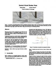
Fig. 1. Scenes rendered with many lights casting shadows at 1920×1080 resolution on an NVIDIA Geforce Titan. From the left: H OUSES with 1.01M triangles and 256 lights (23ms), N ECROPOLIS with 2.58M triangles and 356 lights (34ms), C RY S PONZA with 302K triangles and 65 lights (16ms).

by first fitting projections, or frustums, to shadow receivers and II. P REVIOUS W ORK a) Real Time Many Light Shading: Tiled Shading is a then allocating shadow maps from an atlas texture to match recent technique that supports many thousands of lights in the on-screen shadow frequency. Fitting frustums to shadow real-time applications [4], [1], [2]. In this technique, lights receivers and matching frequency enables high quality and are binned into 2D screen-space tiles that can then be queried memory efficiency. However, by working on a per-object basis, for shading. This is a very fast and simple process, but the the system cannot handle large objects, in particular close to 2D nature of the algorithm creates a strong view dependence, the viewer where a high resolution is required, and irregularly resulting in poor worst case performance and unpredictable shaped objects degrade memory efficiency. In addition, each projection must perform culling and rendering individually, frame times. Clustered Shading extends the technique by considering reducing scalability and producing seams between shadow bins of higher dimensionality, which improves efficiency and maps. King and Newhall [20] describe an approach using cube reduces view dependence significantly [3]. The clusters provide a three-dimensional subdivision of the view frustum, defining maps. They reduce the number of shadow casters rendered by groups, or clusters, of samples with predictable bounds. This testing on an object level whether they cast shadows into the provides an important building block for many of the new view frustum. The effectiveness of the culling is limited by techniques described in this paper, and we review this technique neglecting to make use of information about shadow receivers. Lacking information about receivers also means that, contrary to in Section IV-A. b) Shadow Algorithms: Studies on shadowing techniques Forsyth, they do not attempt to calculate the required resolution. generally present results considering only a single light source, This generally leads to overestimation of the shadow map usually with long or infinite range (e.g., the sun). Consequently, resolution, which combined with the omni-directional nature it is unclear how these techniques scale to many light sources, of cube maps, leads to very high memory requirements. e) Ray Traced Shadows: Recently, Harada et al. [21] whereof a large proportion affect only a few visible samples. For a review of shadow algorithms, refer to the very comprehensive described integrating ray traced shadows into a Tiled Forward books by Eisemann et al. [8] or by Woo and Poulin [9]. The Shading system. They demonstrate that it can be feasible to shadow algorithm which is most relevant to this paper is the ray trace shadows for many lights in a static scene, but do not industry standard Shadow Mapping (SM) algorithm due to report any analysis or comparison to other techniques. While ray tracing can support real-time shadow queries today, the cost Williams [10]. c) Virtual Shadow Maps: Software-based virtual shadow of constructing high-quality acceleration structures put its use maps for single lights have been explored in several publica- beyond the reach of practical real-time use for dynamic scenes. tions, and shown to achieve high quality shadows in bounded Karras and Aila [22] present a comprehensive evaluation of memory [11], [12], [13]. Virtual texturing techniques have the trade-off between fast construction and ray tracing. also long been applied in rendering large and detailed environments [14], [15]. Recently, API and hardware extensions have III. P ROBLEM OVERVIEW been introduced that makes it possible to support virtual textures In this paper, we limit the study to omni-directional point much more conveniently and with performance equalling that lights with a finite sphere of influence (or range) and with of traditional textures [16]. d) Many light shadows: There exists a body of work in some fall-off such that the influence of the light becomes zero the field of real-time global illumination that explores using at the boundary. This is the prevalent light model for real-time many light sources with shadow casting, for example Imperfect applications, as it makes it easy to control the number of lights Shadow Maps [17], and Many-LODs [18]. However, these affecting each part of the scene, which in turn dictates shading techniques assume that a large number of lights affect each performance at run time. Other distributions, such as spotlights sample to conceal approximation artifacts. In other words, these and diffuse lights, can be considered a special case of the approaches are unable to produce accurate shadows for samples omni-light, and the implementation of these types of lights would not affect our findings. lit by only a few lights. Forsyth [19] describes a system that supports several point The standard shadow algorithm for practically all real-time lights that cast shadows. The system works on an object level, rendering is some variation on the classical Shadow-Map (SM) 1077-2626 (c) 2015 IEEE. Personal use is permitted, but republication/redistribution requires IEEE permission. See http://www.ieee.org/publications_standards/publications/rights/index.html for more information.


algorithm. There are many reasons for this popularity, despite 1) Render scene to G-Buffers. the sampling issues inherent in the technique. First, hardware 2) Cluster assignment – calculating the cluster keys of each support is abundant and offers high performance; secondly, view sample. arbitrary geometry is supported; thirdly, filtering can be used to 3) Find unique clusters – finding the compact list of unique produce smooth shadows boundaries; and lastly, no expensive cluster keys. acceleration structure is required. Hence, we explore the design 4) Assign lights to clusters – creating a list of influencing and implementation of a system using shadow maps with many lights for each cluster. lights. To support omni-directional lights, we make use of cube 5) Select shadow map resolution for each light. shadow maps. 6) Allocate shadow maps. 7) Cull shadow casting geometry for each light. In general, the problems that need to be solved when using 8) Rasterize shadow maps. shadow maps with many lights are to: 9) Shade samples. • determine which lights cast any visible shadows, • determine required resolution for each shadow map, • allocate shadow maps, A. Clustered Shading Overview • render shadow casting geometry to shadow maps, and In clustered shading the view volume is subdivided into a grid • shade scene using lights and shadow maps. of self-similar sub-volumes (clusters), by starting from a regular Clustered shading constructs a list of lights for each cluster. 2D grid in screen space, e.g., using tiles of 32 × 32 pixels, A light that is not referenced by any list cannot cast any visible and splitting exponentially along the depth direction. Next, all shadow and is not considered further. Section IV-A provides visible geometry samples are used to determine which of the an overview of the clustered shading algorithm. clusters contain visible geometry. Once the set of occupied Ideally, we should attempt to select a resolution for each clusters has been found, the algorithm assigns lights to these shadow map that ensures the same density of samples in the by intersecting the light volumes with the bounding box of shadow map as of the receiving geometry samples in the frame each cluster. This yields a list of cluster/light pairs, associating buffer. This can be approached if we allow very high shadow- each cluster with all lights that may affect a sample within map resolutions and calculate the required resolution based on (see Fig. 2). Finally, each visible sample is shaded by looking the samples in the frame buffer [13]. We describe our approach up the lights for the cluster it is within and summing their to this problem for many lights in Section IV-B. contributions. For regular shadow maps, storage is tightly coupled with Geometry resolution, and therefore, they cannot be used with a resolution C0 selection scheme that attempts to maintain constant quality. We Occupied Cluster therefore turn to virtual shadow maps, which allow physical Y memory requirements to be correlated with the number of C1 Eye L0 -Z samples requiring shading. Virtual, or sparse, textures have C2 recently become supported by hardware and APIs. We present Near L1 our design of a memory-efficient and high-performance virtual C3 shadow-mapping algorithm in Section IV-C. Cluster/Light Pairs: Rendering geometry to shadow maps efficiently requires Far C1 L0 C2 L0 C2 L1 C3 L1 … culling. When supporting many lights, each light only affects a small portion of the scene, and culling must be performed with Fig. 2. Illustration of the depth subdivisions into clusters and light assignment. a finer granularity than for a single, scene-wide, light. Therefore, Clusters containing some geometry are shown in blue. our algorithm must minimize the amount of geometry drawn to each shadow map. In particular, we should try to avoid The key pieces of information this process yields are a set drawing geometry that does not produce any visible shadow, of occupied clusters with associated bounding volumes (that while at the same time keeping the overhead for culling low. approximate the visible geometry), and the near-minimal set Details of our design for culling shadow casters are presented of lights for each cluster. Intuitively, this information should in Section IV-D. be possible to exploit for efficient shadow computations, and The final step, to shade the scene using the corresponding this is exactly what we aim to do in the following sections. shadow map for each light, is straightforward with modern rendering APIs. Array textures can be used to enable access to B. Shadow Map Resolution Selection many simultaneous shadow maps. See Section IV-F for details. A fairly common way to calculate the required resolution for point-light shadow maps is to use the screen-space coverage IV. BASIC A LGORITHM of the lights’ bounding sphere [20]. While very cheap to Our basic algorithm is shown below. The algorithm is compute, this produces vast overestimates whenever the camera constructed from clustered deferred shading (reviewed in is near, or within, the light volume. To calculate a more Section IV-A), with shadows added as outlined in the previous precisely matching resolution, one might follow the approach in section. Steps that are inherited from ordinary clustered deferred Resolution Matched Shadow Maps (RMSM) [13], and compute shading are shown in gray. shadow-map space derivatives for each view sample. However, 1077-2626 (c) 2015 IEEE. Personal use is permitted, but republication/redistribution requires IEEE permission. See http://www.ieee.org/publications_standards/publications/rights/index.html for more information.


C. Shadow Map Allocation

Cluster

α Light Source (a)

(b)

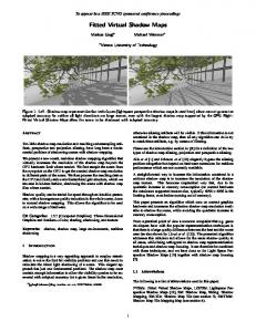
Fig. 3. (a), the solid angle of cluster, with respect to the light source, α, subtended by the cluster, illustrated in 2D. (b), example of undersampling due to an oblique surface violating assumptions in Equation 1, shown with and without textures and PCF.

applying this na¨ıvely would be expensive, as the calculations must be repeated for each sample/light pair and requires derivatives to be stored in the G-Buffer. Our goal is not to attempt alias-free shadows, but to quickly compute a reasonable estimate. Therefore, we base our calculations on the bounding boxes of the clusters, which are typically several orders of magnitude fewer than the samples. The required resolution, R, for each cluster is estimated as the number of pixels covered by the cluster in screen space, S, divided by the proportion of the unit sphere subtended by the solid angle, α, of the cluster bounding sphere, and distributed over the six cube faces (see Fig. 3(a) and Equation 1).

Using the resolutions computed in the previous step, we can allocate one virtual cube shadow map for each light with a non-zero resolution. This does not allocate any actual physical memory backing the texture, just the virtual range. In virtual textures, the pages are laid out as tiles of a certain size (e.g., 256 × 128 texels), covering the texture. Before we can render into the shadow map we must commit physical memory for those pages that will be sampled during shading. The pages to commit could be established by projecting each sample onto the cube map, i.e., performing a shadow lookup, and recording the requested page. Again, the cost can be reduced substantially by using cluster/light pairs in place of sample/light pairs. This requires projecting the cluster bounding boxes onto the cube maps, which is more complex than point lookups (see Fig. 4). Fortunately, by transforming the cluster bounding box to the same space as the cube map, we arrive at very simple calculation (see Listing 1). This transformation is conservative, but as the cluster bounding boxes are roughly cube shaped by design, the bounding box inflation is acceptable. We calculate the projection for each cluster/light pair and build up a mask for each light representing the affected tiles that we call the virtual-page mask.

D. Culling Shadow-Casting Geometry

Culling is a vital component of any real time rendering system and refers to the elimination of groups, or batches of r triangles that are outside a viewing volume. This is typically S/(α/4π) (1) achieved by querying an acceleration structure representing R= 6 the scene geometry with the view volume. Intuitively, effective This calculation is making several simplifying assumptions. culling requires some correlation between the size of the view The most significant is that we assume that the distribution of volume and the geometry batches. If the batches are too large, the samples is the same in shadow-map space as in screen space. many triangles that are outside the view volume will be drawn. In our application, the view volumes are the bounding This leads to an underestimate of the required resolution when spheres of the lights. These volumes are much smaller than the light is at an oblique angle to the surface (see Fig. 3(b)). what is common for a primary view frustum, and therefore A more detailed calculation might reduce these errors, but requires smaller triangle batches. To explore this, we make we opted to use this simple metric, which works well for the use of a bounding volume hierarchy (BVH), storing triangle majority of cases. batches at the leaves. Each batch has an axis aligned bounding For each cluster/light pair, we evaluate Equation 1 and retain box (AABB), which is updated at run time, and contains a fixed the maximum R for each light as the shadow map resolution, maximum number of triangles. By changing the batch size we i.e., a cube map with faces of resolution R × R. can explore which granularity offers the best performance for our use case. The hierarchy is queried for each light, producing a list of batches to be drawn into each cube shadow map. For each element, we also store a mask with six bits that we call the cube-face mask (CFM), which indicates which cube faces the batch must be drawn into. See Fig. 5 for a two-dimensional illustration.

Fig. 4. The projected footprint (purple) of an AABB of either a batch or a cluster (orange), projected onto the cube map (green). The tiles on the cube map represent either virtual texture pages or projection map bits, depending on application.

E. Rasterizing Shadow Caster Geometry The best way to render the batches to the shadow maps is mostly down to implementation details. Our design is covered in Section VI-D.



Batch Hierarchy Cube Culling Planes

Light Sphere

…

{CFM, batch index}…

1

2

…

Fig. 5. Illustration of batch hierarchy traversal. The AABBs of batches 1 and 2 intersect the light sphere, and are tested against the culling planes, which determine the cube faces the batch must be rendered to.

B. Non-uniform Light Sizes The resolution selection presented in Section IV-B uses the maximum sample density required by a cluster affected by a light. If the light is large and the view contains samples requiring very different densities, this can be a large overestimate. This occurs when a large light affects not only some, relatively few, samples nearby the viewer but also a large portion of the visible scene further away (see Fig. 6). The nearby samples dictate the resolution of the shadow map, which then must be used by all samples. The result is oversampling for the majority of the visible samples and a high storage cost.

F. Shading Shading is computed as a full-screen pass. For each sample, the shader loops over the list of lights in the cluster and accumulates shading. To sample shadow maps we use the index of the light to also look up a shadow map. Using a texture array with cube maps this is can simply be a direct mapping. However, to enable many simultaneous cube shadow maps with different resolutions is somewhat more complex, see Section VI-C for implementation details. V. A LGORITHM E XTENSIONS In the previous section we detailed the basic algorithm. This section presents a number of improvements and extensions which expand the efficiency and capacity of the algorithm to handle more complex scenes. A. Projection Maps To improve culling efficiency the system should avoid drawing geometry into unsampled regions of the shadow map. In other words, we require something that identifies where shadow receivers are located. This is similar in spirit to projection maps, which are used to guide photon distribution in photon maps, and we adopt this name. Fortunately, this is the same problem as establishing the needed pages for virtual textures (Section IV-C), and we reuse the method of projecting AABBs onto the cube faces. To represent the shadow receivers, each cube face stores a 32 × 32 bit mask (in contrast to the virtual page masks, which vary with resolution), and we project the bounding boxes of the clusters as before. We then perform the same projection for each batch AABB that was found during the culling, to produce a mask for each shadow caster. If the logical intersection between these two masks is zero for any cube face, we do not need to draw the batch into this cube face. In addition to testing the mask, we also compute the maximum depth for each cube face and compare these to the minimum depth of each batch. This enables discarding shadow casters that lie behind any visible shadow receiver. For each batch, we update the cube-face mask to prune non-shadowing batches.

Fig. 6. Illustration of light requiring different sample densities within the view frustum. The nearby, high density, clusters dictate the resolution for the entire light.

If there are only uniformly sized lights and we are comfortable with clamping the maximum allowed resolution, then this is not a significant problem. However, as our results show, if we have a scene with both large and small lights, then this can come to dominate the memory allocation requirements (see Fig. 16). To eliminate this issue, we allow each light to allocate a number of shadow maps. We use a fixed number, as this allows fast and simple implementation, in our tests ranging from 1 to 16 shadow maps per light. To allocate the shadow maps, we add a step where we build a histogram over the resolutions requested by the clusters affected by each light. The maximum value within each histogram bucket is then used to allocate a distinct shadow map. When the shadow-map index is established, we replace the light index in the cluster light list with this index. Then, culling and drawing can remain the same, except that we sometimes must take care to separate the light index from the shadow-map index. C. Level of Detail For high-resolution shadow maps that are used for many view samples, we expect that rasterizing triangles is efficient, producing many samples for each triangle. However, lowresolution shadow maps sample the shadow-casting geometry sparsely, generating few samples per triangle. To maintain efficiency in these cases, some form of Level of Detail (LOD) is required. In the limit, a light might only affect a single visible sample. Thus, it is clear that no amount of polygon-based LOD will suffice by itself. Consequently, we explore the use of ray tracing, which enable efficient random access to scene geometry. To



Light/Cluster Pairs

Cluster Generation + Light Assignment

Cluster Bounds

Batch List

Build Projection Maps

Shadow Map Resolution Calc

SM Resolutions Virtual Page Mask Calc

Projection Maps

Page Masks

Batch AABBs

Cull Batches

SM/Batch ID + Face Mask Pairs

Model

Build Batch Hierarchy

Batch Hierarchy

Batch Counts + Offsets / SM

Render Model

G-Buffers

Update Batch AABBs

Build Shadow Map Projections

SM Projection Matrices

Render Batches

Allocate Shadow Maps

Shadow Map Render Targets

Shadow Maps

Build Draw Commands

Draw Commands

Final Image

Light List

Compute Shading (Ray Trace) Lighting Composit

Fig. 7. Stages (rounded) and data (square) in the algorithm implementation. Stage colors correspond to those used in Fig. 12. All computationally demanding stages are executed on the GPU, with sequencing and command issue performed by the CPU.

decide when ray tracing should be used, we simply use a threshold (in our tests we used 96 texels as the limit) on the resolution of the shadow map. Those shadow maps that are below the threshold are not further processed and are replaced by directly ray tracing the shadows in a separate shading pass. We refer to this as the hybrid algorithm. We also evaluate using ray tracing for all shadows to determine the cross-over point in efficiency versus shadow maps. Since we aim to use the ray tracing for LOD purposes, we chose to use a voxel representation, which has an inherent polygon-agnostic LOD and enables a much smaller memory footprint than would be possible using triangles. We use the technique described by Kämpe et al. [23], which offers performance comparable to state of the art polygon ray tracers and has a very compact representation. A key difficulty with ray tracing is that building efficient acceleration structures is still a relatively slow process, at best offering interactive performance, and dynamically updating the structure is both costly and complex to implement [22]. We therefore only explore using a static acceleration structure, enabling correct occlusion from the static scene geometry, which often has the highest visual importance. As we aim to use the ray tracing for lights far away (and therefore low resolution), we consider this a practical use case to evaluate. For highly dynamic scenes, our results that use ray tracing are not directly applicable. Nevertheless, by using a high-performance accelerations structure, we aim to explore the upper bound for potential ray tracing performance. To explore the use of polygon-based LOD, we constructed a low-polygon version of the H OUSES scene (see Section VII). This is done in lieu of a full blown LOD system to attempt to establish an upper bound for shadow-mapping performance when LOD is used. D. Exploiting Static Scene Elements The system for shadow maps presented thus far is entirely dynamic, and makes no attempts to exploit that part of the scene is static. In practice, coherent and gradually changing views combined with static lights and geometry is quite common in many scenes. In addition, modern shading approaches, like tiled and clustered shading, require that all the shadow maps must exist before the shading pass. This makes it very easy to preserve the contents of the shadow maps between frames, at no additional storage cost.

To explore this, our aim is to avoid drawing any geometry that will not produce any change in the shadow map. We can discard any batch which meets the below criteria. 1) The light is static. 2) The batch is static. 3) The batch was drawn last frame. 4) The batch projection does not overlap that of any dynamic batch drawn the previous frame. 5) The batch projection does not overlap any virtual page that is committed this frame. 6) The shadow-map resolution is unchanged. The first step is to simply flag lights and batches as dynamic or static, which can be done based on the scene animation. Next we must detect whether a batch was drawn into a shadow map the previous frame, which is done by testing overlap against the projection map from the previous frame. To test conditions 4 and 5 efficiently, we construct a mask with a bit set for any part of the shadow map that needs to be cleared, i.e., either freshly committed or containing dynamic geometry the last frame. All bits in this mask are set if the resolution has changed, which means everything must be drawn. These conditions and masks are tested in addition to the projection map as described in Section V-A. Finally, we must also clear the regions of the shadow map marked in the clear mask. This is not directly supported by any existing rendering API, and we therefore generate and draw point sprites at the far plane, with the depth test set to pass anything. Note that to support batches that transition between dynamic and static status over time requires special care. If a batch changes status from static to dynamic, then it will not be in the dynamic map of the previous frame, and therefore the region may not be cleared correctly. In our implementation, the status is simply not allowed to change. Lights, however, are allowed to change status. E. Explicit Cluster Bounds As clusters are defined by a location in a regular grid within the view frustum, there is an associated bounding volume that is implied by this location. Computing explicit bounds, i.e., tightly fitting the samples within the cluster, was found by Olsson et al. [3] to improve light-culling efficiency, but it also incurred too much overhead to be worthwhile. When



introducing shadows and virtual shadow map allocation, there is more to gain from tighter bounds. We therefore present a novel design that computes approximate explicit bounds with Light Backfacing very little overhead on modern GPUs. We store one additional 32-bit integer for each cluster, which is logically divided into three 10-bit fields. Each of these Light Frontfacing represent the range of possible positions within the implicit AABB. With this scheme, the explicit bounding box can be constructed using a single 32-bit atomicOr reduction for each sample. To reconstruct the bounding box, we make use of intrinsic bit-wise functions to count zeros from both directions in each Fig. 9. Backface culling of lights. The fragments generated by the vertical wall 10-bit field, see __clz and __ffs in Fig. 8. These bit positions (purple box) are back-facing with respect to the light source. Normal clustering are then used to resize the implicit AABB in each axis direction. can detect this, and will not assign the light to these clusters (despite their __clz

__ffs

bounding volumes overlapping the light’s bounding sphere). No shadow maps are requried in the direction of these clusters, unless other light front-facing clusters (red box) project to the same parts of the shadow map.

0 1 0 1 1 0 0 0 0 0 0 0 0 0 1 1 1 0 0 0

A. Shadow Map Resolution Selection

Explicit Implicit

Fig. 8. The computation of explicit bounds, illustrated in 2D. __clz and __ffs are the CUDA operations Count Leading Zeroes and Find First Set.

The implementation of shadow-map resolution selection is a set of CUDA kernels, launched with one thread per cluster/light pair. These kernels compute the resolution, cube-face mask, virtual-page mask, and also the projection map, for each shadow map. To reduce the final histograms and bit masks, we use atomic operations, which provide adequate performance for current GPUs. The resulting array of shadow-map resolutions and the array of virtual-page masks are transferred to the CPU using an asynchronous copy. For details on the projection see Appendix A.

F. Backface Culling Olsson et al. [3] explore clustering based on both position and normal direction of fragments. By testing a normal cone in addition to the bounding box, lights can be removed from clusters that face away from the light. While they observed a significant reduction in the number of lighting computations, the overhead arising from the increased number of clusters due to the normal clustering, overshadow the gains in shading performance. With shadows, which introduce much higher total cost for each shaded sample, the potential performance improvements are correspondingly greater. Culling additional lights would not only reduce the number of lights that are to be considered during shading, but also potentially the number of shadow map texels that need to be stored. There is no need to store shadow maps towards surfaces that are back-facing with respect to a light source (illustrated in Fig. 9), unless other visible light– front-facing surfaces project to the same parts of the shadow map. VI. I MPLEMENTATION We implemented the algorithm and variants above using OpenGL and CUDA. All computationally intensive stages are implemented on the GPU, and in general, we attempt to minimize stalls and GPU to CPU memory transfers. However, draw calls and rendering state changes are still necessary to invoke from the CPU, and thus, we must transfer some key information from the GPU. The system is illustrated in Fig. 7.

B. Culling Shadow-Casting Geometry In the implementation, we perform culling before allocating shadow maps, as this allows a greater degree of asynchronous overlap, and also minimizes transitions between CUDA and OpenGL operation. 1) Batch Hierarchy Construction: Each batch is a range of triangle indices and an AABB, constructed such that all the vertices share the transformation matrix1 and are located close together, to ensure coherency under animation. The batches are created off-line, using a bottom-up agglomerative treeconstruction algorithm over the scene triangles, similar to that described by Walter et al. [24]. Unlike them, who use the surface area as the dissimilarity function, we use the length of the diagonal of the new cluster, as this produces more localized clusters (by considering all three dimensions). After tree construction, we create the batches by gathering leaves in sub-trees below some predefined size, e.g., 128 triangles (we tested several sizes, as reported below). The batches are stored in a flat array and loaded at run time. At run time, we re-calculate each batch AABB from the transformed vertices every frame to support animation. The resulting list is sorted along the Morton curve, and we then build an implicit left balanced 32-way BVH by recursively grouping 32 consecutive AABBs into a parent node. This is the same type of hierarchy that was used for hierarchical 1 We only implement support for a single transform per vertex, but this is trivially extended to more general transformations, e.g., skinning.



light assignment in clustered shading, and has been shown to perform well for many light sources [3]. 2) Hierarchy Traversal: To gather the batches for each shadow map, we launch a kernel with a CUDA block for each shadow map. The reason for using blocks is that a modern GPU is not fully utilized when launching just a warp per light (as would be natural with our 32-way trees). The block uses a cooperative depth-first stack to utilize all warps within the block. We run this kernel in two passes to first count the number of batches for each shadow map and allocate storage, and then to output the array of batch indices. In between, we also perform a prefix sum to calculate the offsets of the batches belonging to each shadow map in the result array. We also output the cube-face mask for each batch. This mask is the bitwise and between the cube-face mask of the shadow map and that of the batch. The counts and offsets are copied back to the CPU asynchronously at this stage, as they are needed to issue drawing commands. To further prune the list of batches, we launch another kernel that calculates the projection-map overlap for each batch in the output array and updates the cube-face mask (see Section V-A). If static geometry optimizations are enabled, this kernel performs the tests described in Section V-D, and also builds up the projection map containing dynamic geometry for next frame. The final step in the culling process is to generate a list of draw commands for OpenGL to render. We use the OpenGL 4.3 multi-draw indirect feature (glMultiDrawElementsIndirect), which allows the construction of draw commands on the GPU. We map a buffer from OpenGL to CUDA and launch a kernel where each thread transforms a batch index and cube-face mask output by the culling into a drawing command. The vertex count and offset is provided by the batch definition, and the instance count is the number of set bits in the cube-face mask.

virtual 2D-array texture. At run time, we allocate chunks of six layers from this to act as cube shadow maps as needed. We allocate the maximum resolution as all layers must have the same size, and use just the portion that is required to support the resolution of the given shadow map. This precludes using hardware supported cube shadow lookup, as this maps the direction vector to the entire texture surface. Instead, we implement the face selection and 2D coordinate conversion manually in the shader. The overhead for this is small, on modern hardware. However, using array textures we are currently limited to b2048/6c shadow maps, where 2048 is the maximal number of layers supported by most OpenGL drivers. In previous work this limitation was avoided by using so called bindless textures, which enable limitless numbers of textures. Unfortunately, random accessing bindless textures is not allowed by the standard, and was found to be very slow on NVIDIA hardware (see Fig. 14). D. Rasterizing Shadow Caster Geometry

With the set up work done previously, preparing drawing commands in GPU-buffers, the actual drawing is straightforward. For each shadow map, we invoke glMultiDrawElementsIndirect once, using the count and offset shipped back to the CPU during the culling. To route the batches to the needed cube map faces, we use layered rendering and a geometry shader. The geometry shader uses the instance index and the cube-face mask (which we supply as a per-instance vertex attribute) to compute the correct layer. The sparse textures, when used as a frame buffer target, quietly drop any fragments that end up in uncommitted areas. This matches our expectations well, as such areas will not be used for shadow look ups. Compared to previous work on software virtual shadow maps, this is an enormous advantage, as we sidestep the issues of fine-grained binning, clipping and copying and also do not have to allocate temporary rendering buffers. C. Shadow Map Allocation We did not implement support for different materials (e.g., To implement the virtual shadow maps, we make use to support alpha masking). To do so, one draw call per shadow of the OpenGL 4.4 ARB extension for sparse textures material type would be needed instead. (ARB_sparse_texture). The extension exposes vendor1) Workarounds: When rendering to sparse shadow maps, specific page sizes and requires the size of textures with sparse we expected that clearing the render target should take time storage to be multiples of these. On our target hardware, the proportional to the number of committed pages. However, we page size is 256 × 128 texels for 16-bit depth textures (i.e., observed cost proportional to the size of the render target 64kb), which means that our square cube-map faces must be (despite setting both viewport and scissor rectangle). This was aligned to the larger value. For our implementation, the logical particularly as all render targets in our 2D-array are of the maxipage granularity is therefore 256×256 texels, which also limits mum resolution. Furthermore, using glClearTexSubImage to the maximum resolution of our shadow maps to 8K×8K texels, clear just the used portion exhibited even worse performance. as we use up to 32 × 32 bits in the virtual-page masks. The best performing workaround we found was to draw Thus, for each non-zero value in the array of shadow map a point sprite covering each committed page, which offered resolutions, we round the requested resolution up to the next consistent and scalable performance. This is an area where page boundary and then use this value to allocate a texture future drivers ought to be able to offer improved performance, with virtual storage specified. Next, we iterate the virtual-page by clearing only what is committed. mask for each face and commit physical pages. If the requested resolution is small, in our implementation below 64 × 64 texels, VII. R ESULTS AND D ISCUSSION we use an ordinary physical cube map instead. In practice, creating and destroying textures is a slow All experiments were conducted on an NVIDIA GTX Titan operation in OpenGL, and we therefore create just a single GPU. We used three scenes (see Fig. 1). H OUSES is designed 1077-2626 (c) 2015 IEEE. Personal use is permitted, but republication/redistribution requires IEEE permission. See http://www.ieee.org/publications_standards/publications/rights/index.html for more information.


60 50

RayTrace

Hybrid

PMCD-EB

PMCD-EB-Pcf

PMCD-EB-LOD

PMCD-EB-SO

40

Time [ms]

CFM

30 20 10

90

18

80

16

70

14

60

12

50

10

40

8

30

6

20

4

10

2

0

0 0

100

200

(a) H OUSES.

300

0

0

100

200

(b) N ECROPOLIS.

300

0

100

200

300

(c) C RY S PONZA.

Fig. 10. Wall-to-wall frame times from the scene animations, for different algorithm variations. The times exclude time to commit physical memory. For all except ’PMCD-EB-SO’ this is achieved by measuring each frame multiple times and retaining the median time. As ’PMCD-EB-SO’ makes use of frame to frame coherency, we instead subtract the time to commit physcal memory measured.

this overhead from our measurements, unless otherwise stated, as it introduces too much noise and does not represent useful work. All reported figures are using a batch size of up to 128 triangles. We evaluated several other batch sizes and found that performance was similar in the range 32 to 512 triangles per batch, but was significantly worse for larger batches. This is expected, as larger batches lead to more triangles being drawn, and rasterization is already a larger cost than culling in the algorithm (see Fig. 12). a) Performance: We report the wall-to-wall frame times 3000 60 for our main algorithm variants in Fig. 10. These are the times #Commits between consecutive frames and thus include all rendering 2500 50 Cost/Commit activity needed to produce each frame, as well as any stalls. 2000 40 From these results, it is clear that virtual shadow maps with projection-map culling offer robust and scalable performance 1500 30 and that real-time performance with many lights and dynamic 1000 20 scenes is achievable. Comparing these to the breakdown in Fig. 12, where individual stages are measured, we see that for 500 10 the lighter scenes (Fig. 12(f)), a greater proportion of the time 0 0 is lost to stalls, leaving room for performance improvements 0 100 200 300 with better scheduling. Fig. 12(d) demonstrates that well over Fig. 11. Number of pages commited and cost of each call over the 30 FPS is achievable in N ECROPOLIS , if all stalls and other N ECROPOLIS animation. overheads were removed (for example switching render targets We evaluate several algorithm variants with different modifi- and similar), and C RY S PONZA could run at over 100 FPS with cations: Shadow maps with projection map culling (PMC), and 65 lights. As expected, ray tracing offers better scaling when the shadwith added depth culling (PMCD); with explicit bounds (EB); ows require fewer samples, with consistently better performance with static geometry optimizations (SO); with normal clustering in the first part of the zooming animations in N ECROPOLIS (Nk); only using cluster face mask culling (CFM); Ray Tracing; and H OUSES (Fig. 10). When the lights require more samples, and Hybrid, which uses PMCD-EB. Unless otherwise indicated, shadow maps generally win, and also provide better quality, four cube shadow maps per light is used. For the normal as the voxel representation used for ray tracing is quite coarse. clustering, we report times for using 3 × 3 directions per The hybrid method is able to make use of this advantage cube face. This corresponds to the Nk3 clustering by Olsson and provides substantially better performance early in the et al. [3] (we do not compute explicit bounding cones in this N ECROPOLIS animation (Fig. 12(c)). However, it fails to implementation). improve worst-case performance because there are always a Committing physical storage is still relatively slow and 2 few small lights visible, and our implementation runs a separate unpredictable on current drivers . Fig. 11, shows that the full-screen pass in CUDA to shade these. Thus, efficiency in average cost is quite low, 7µs, and usable for real-time these cases is low, and we would likely see better results if applications. However, the peak cost coincides with the highest the ray tracing better integrated with the other shading. An commit rates, perhaps indicating some issue with batching or improved selection criterion, based on the estimated cost of coherency in the driver. This leads to large spikes, up to over the methods rather than just shadow-map resolution, could also 100ms, just to commit physical memory. We therefore subtract improve performance. For example, the LOD version of the 2 The NVIDIA driver version 344.65 was used in our measurements. H OUSES scene (Fig. 10(a)) highlights that the cost of shadow Time [µs]

Count

to be used to illustrate the scaling in a scene where all lights have a similar size and uniform distribution. N ECROPOLIS is derived from the Unreal SDK, with some lights moved slightly and all ranges doubled. We added several animated cannons shooting lights across the main central area, and a number of moving objects. The scene contains 275 static lights and peaks at 376 lights. C RY S PONZA is derived from the Crytek version of the Sponza atrium scene, with 65 light sources added. Each scene has a camera animation, which is used in performance graphs (see the supplementary video).



45 Shading

40

DrawShadowMaps

CullBatches

35

LightAssignment

30 Time [ms]

FindUniqueClusters RenderModel

25 20 15 10

5 0 0

100

200

0

300

100

(a) Shadow Maps (PMCD-EB). 45

Shading ClearSM LightAssignment RenderModel

40 35

DrawShadowTris CullBatches FindUniqueClusters

30

200

300

100

200

300

(c) Hybrid (PMCD-EB).

45

10

40

9

35

8 7

30

Time [ms]

0

(b) Ray Tracing.

6

25

25

20

20

15

15

10

10

2

5

5

1

0

0

5

0

100

200

300

(d) PMCD-EB - Without overhead.

4 3

0

0

100

200

300

(e) PMCD-EB-SO - Without overhead.

0

100

200

300

(f) C RY S PONZA PMCD-EB - Without overhead.

Fig. 12. Performance timings broken down into the principal stages of the algorithms, measured individually, from the N ECROPOLIS scene animation, for different algorithms. Note that for (b) and (c), the ray tracing time forms part of the shading. Bottom row shows the breakdown with further non-intrinsic overhead removed, e.g., the cost for switching render targets.

mapping is correlated to the number of polygons rendered. The Similar to the results of Olsson et al. [3], any performance LOD version also demonstrates that there exists a potential for gains from back-face culling with normal clustering are offset performance improvements using traditional polygon LOD, as by the overheads incurred from performing the finer clustering an alternative or in addition to ray tracing. and working with the additional clusters during the different The largest cost in the batch culling comes from updating phases of the method. The reason that the relatively large the batch AABBs and re-building the hierarchy (Fig. 13). reduction in lighting computations shown in Fig. 16 fails to In practice, these costs can be reduced significantly as only translate into large performance improvements, is that those dynamic geometry needs to be updated, rather than all scene are the lights that will be discarded after an initial back-facing geometry as done in our implementation. The static geometry test in the shader, before any expensive operations. optimizations implement the former of this optimizations BatchHierarchyTraverse UpdateBatches BuildBatchHierarchy as well as reducing the number of triangles drawn. This CalcShadowMapRes ClearBuffers ProjectionMapCull yields substantial performance improvements in H OUSES BuildCubeMapProjections and N ECROPOLIS, while for the C RY S PONZA scene any improvement is likely absorbed by stalls. Fig. 12(e) shows 11% 15% 17% 18% 19% 7%7% 7% the breakdown of this optimization for N ECROPOLIS, demon5% 3% 8% 7% 19% 14% 1% 18% 49% 12% 5% 27% 14% strating large improvements in triangle drawing times overall, 3% 2% 1% 49% 27% and a small increase in batch culling cost due to the added 28% steps to compute the new masks. Worst case performance is not improved significantly, indicating that in this part of the N ECROPOLIS (3.5ms) H OUSES (2.0ms) C RY S PONZA (1.8ms) animation the cost is dominated by dynamic lights and objects. Shading performance (Fig. 14) depends on several factors. Fig. 13. Timing breakdown of the steps involved in culling batches. The displayed percentage represents the maximum time for each of the steps over The use of bindless textures with incoherent accesses can the entire animation. be expensive. The switch to a 2D array texture, yields a significant performance improvement, especially of the worst Shadow filtering, in our implementation a simple nine-tap case. Incoherent access is still an issue, though much less Percentage-Closer filter (PCF), makes up a sizeable proportion significant, and is unfortunately increased when using normal of the total cost, especially in the scenes with relatively many cone culling. Some improvement can be seen from reordering lights affecting each sample (Fig. 10). Thus, techniques that the light lists to increase coherency. reduce this cost, for example using pre-filtering, could be a Although the back-face culling reduces the shading time in useful addition. some parts, it increases when many shadow maps are active. b) Culling Efficiency: Culling efficiency is greatly imWe suspect that this is again due to incoherent shadow map proved by our new methods exploiting information about accesses, where the problem is exacerbated by the larger shadow receivers inherent in the cluster, as shown in Fig. 15. number of smaller clusters arising from normal clustering. Compared to na¨ıvely culling using the light sphere and drawing 1077-2626 (c) 2015 IEEE. Personal use is permitted, but republication/redistribution requires IEEE permission. See http://www.ieee.org/publications_standards/publications/rights/index.html for more information.


significant, since most lights are found in the large main areas of the our test scenes - which is also where the camera passes 7 PMCD-EB-NK3 through. PMCD-EB-PCF 6 c) Memory Usage: As expected, using only a single PMCD-EB-NK3-PCF 5 shadow map per light has a very high worst case cost PMCD-EB-NK3-LR-PCF 4 for N ECROPOLIS, which contains a few very large lights, 3 (Fig. 16:’PMCD-EB-1SM’). With four shadow maps per light, 2 we get a better correspondence between lighting computations 1 (i.e., the number of light/sample pairs shaded) and number of shadow-map texels allocated. This indicates that peak 0 0 100 200 300 shadow-map usage is correlated to the density of lights in Fig. 14. Shading performance for different methods. We also show mea- the scene, which is a very useful property when budgeting surements when reordering the light lists such that fragments from a single rendering resources. The largest number of shadow-map texels screen-space tile access shared lights in the same order (‘-LR’). per lighting computation occurs when shadow maps are low resolution, early in the animation, and does not coincide with to all six cube faces, our method is always at least six times peak memory usage. We tested up to 16 shadow maps per light, and observed that above four, the number of texels rises more efficient. When adding the max-depth culling for each cube face, again. The best value is likely to be scene dependent. The back-face culling using the normal clustering results, the additional improvement is not as significant. This is not unexpected as the single depth is a very coarse representation, as predicted, in a slight reduction in the number of shadow most lights are relatively short range, and the scene is mostly map texels (Fig. 16) that need to be allocated. The contrast open with little occlusion. Towards the end of the animation, between the substantial reduction in Lighting Computations where the camera is inside a building, the proportion that is and the modest reduction in committed texels indicates that culled by the depth test increases somewhat. The cost of adding the problem illustrated in Fig. 9 is common in our test scenes. d) Explicit bounds: The explicit bounds provide improved this test is very small (see Fig. 13: ’ProjectionMapCull’). Adding the static scene element optimizations (Section V-D) efficiency for both the number of shadow-map texels alloimproves efficiency significantly across the relatively smooth cated and number of triangles drawn by 8 − 35% over the camera animation. Despite a large proportion of dynamic lights N ECROPOLIS animation. The greatest improvement is seen in the most intensive part of the animation, peak triangle rate near the start of the animation, where many clusters are is reduced by around 40 percent. This demonstrates that this far away and thus have large implicit bounds in view space approach has a large potential for improving performance in (see Fig. 15). The overhead for the explicit bounds reduction many cases. However, as with all methods exploiting frame- roughly doubles the cost of finding unique clusters. While an to-frame coherency, for rapidly changing views there is no improvement over previous work, yet higher performance for improvement. Our system is oriented towards minimal memory full-precision explicit bounds was recently demonstrated by usage, releasing physical pages as soon as possible. This means Sintorn et al. [25]. e) Quality: As shown in Fig. 3(b), sampling artifacts that higher efficiency could potentially be achieved by retaining physical memory in static areas for longer, especially when occur due to our choice of resolution calculations. However, as we recalculate the required resolutions continuously and select shadow maps are small. the maximum for each shadow map, we expect these errors 20 to be stable and consistent. In the supplementary video, it is PMCD 18 difficult to notice any artifacts caused by switching between CFM 16 PMC-EB shadow-map resolutions. PMCD-EB 14 The cost of calculating the estimated shadow-map resolution PMCD-EB-NK3 12 Hybrid is a very small part of the frame time (Fig. 13). Therefore, PMCD-EB-SO 10 it could be worthwhile exploring more complex methods, to 8 improve quality further. 6 We also added a global parameter controlling undersampling 4 to enable trading visual quality for lower memory usage (see 2 Fig. 16). This enables a lower peak memory demand with 0 0 100 200 300 uniform reduction in quality. For a visual comparison, see the supplementary video. Fig. 15. Triangles drawn each frame in the N ECROPOLIS animation with 9

PMCD-EB-bindless PMCD-EB

Millions

Time [ms]

8

different culling methods. The na¨ıve method, that is, not using the information about clusters to improve culling, is not included in the graph to improve presentation. It renders between 40 and 126 million triangles per frame and never less than six times the number of PMCD.

The back-face culling using the normal clustering results in a slight reduction in the number triangles that need to be drawn (Fig. 15). The reductions are measurable but not very

VIII. C ONCLUSION We presented several new ways of exploiting the information inherent in the clusters, provided by clustered shading, to enable very efficient and effective culling of shadow casting geometry. With these techniques, we have demonstrated that


This article has been accepted for publication in a future issue of this journal, but has not been fully edited. Content may change prior to final publication. Citation information: DOI 10.1109/TVCG.2015.2418772, IEEE Transactions on Visualization and Computer Graphics

450

50

PMCD-EB-1SM PMCD-EB PMCD-EB-U2 PMCD-EB-U4 PMCD-EB-NK3 LightingComputations LightingComputations-NK3

400

350 300 250

45 40

35 30 25

200

20

150

15

100

10

50

5

0

0 0

100

200

300

Millions #SM Texels / Lighting Computation

Millions

12

25 PMCD-EB-1SM PMCD-EB

20

PMCD-EB-U2

PMCD-EB-U4 15

10

5

0 0

100

200

300

Fig. 16. Allocated shadow-map texels for various scenarios over the N ECROPOLIS animation. Shows the performance with a varying number of shadow maps per light, the effect of the global undersampling parameter (u2|u4 suffix), and also plots the number of Lighting Computations for each frame (secondary axis). The number of Lighting Computations is lower for the Nk3-method.

using hardware-supported virtual cube shadow maps is a viable method for achieving high-quality real-time shadows, scaling to hundreds of lights. In addition, we show that memory requirements when using virtual cube shadow maps as described in this paper is roughly proportional to the number of shaded samples. This is again enabled by utilizing clusters to quickly determine both the resolution and coverage of the shadow maps. We also demonstrate that using ray tracing can be more efficient than shadow maps for shadows with few samples and that a hybrid method building on the strength of both is a promising possibility. The implementation of ARB_sparse_texture used in our evaluation does offers real-time performance for many cases, but is not yet stable. However, we expect that future revisions, perhaps combined with new extensions, will continue to improve performance. In addition, on platforms and modern APIs with more direct control over resources, such as game consoles, this problem should be greatly mitigated. The limitation of the number of array texture layers to 2048 limits future scalability of the approach using a global 2D array. This restriction will hopefully be lifted for virtual array textures in the future. Alternatively, bindless textures offer a straightforward solution but is currently hampered by the requirement of coherent access and lower performance. Again, future hardware may well improve performance and capabilities to make this a viable alternative.

IX. F UTURE W ORK In the future, we would like to explore even more aggressive culling schemes, for example using better max-depth culling. We also would like to explore other light distributions, which might be supported by pre-defined masks, yielding high flexibility in distribution. Further exploiting information about static geometry and lights could be used to improve performance, in particular by retaining static information for longer – trading memory for performance. There also seems to exist a promising opportunity to apply the techniques described to global shadow maps, replacing the commonly used cascaded shadow maps. As noted, a more detailed estimation of the required resolution could improve visual quality in some cases.

ACKNOWLEDGEMENTS The Geforce GTX Titan used for this research was donated by the NVIDIA Corporation. We also want to acknowledge the anonymous reviewers for their valuable comments, and Jeff Bolz, Piers Daniell and Carsten Roche of NVIDIA for driver support. This research was supported by the Swedish Foundation for Strategic Research under grant RIT10-0033, and by the People Programme (Marie Curie Actions) of the European Union’s Seventh Framework Programme (FP7) under REA Grant agreement no. 290227 (DIVA). R EFERENCES [1] O. Olsson and U. Assarsson, “Tiled shading,” Journal of Graphics, GPU, and Game Tools, vol. 15, no. 4, pp. 235–251, 2011. [Online]. Available: http://www.tandfonline.com/doi/abs/10.1080/2151237X.2011.621761 [2] T. Harada, “A 2.5D culling for forward+,” in SIGGRAPH Asia 2012 Technical Briefs, ser. SA ’12. ACM, 2012, pp. 18:1–18:4. [Online]. Available: http://doi.acm.org/10.1145/2407746.2407764 [3] O. Olsson, M. Billeter, and U. Assarsson, “Clustered deferred and forward shading,” in Proc., ser. EGGH-HPG’12, 2012, p. 87–96. [Online]. Available: http://dx.doi.org/10.2312/EGGH/HPG12/087-096 [4] M. Swoboda, “Deferred lighting and post processing on PLAYSTATION 3,” Game Developer Conference, 2009. [Online]. Available: http://www.technology.scee.net/files/presentations/gdc2009/ DeferredLightingandPostProcessingonPS3.ppt [5] A. Ferrier and C. Coffin, “Deferred shading techniques using frostbite in ”battlefield 3” and ”need for speed the run”,” in Talks, ser. SIGGRAPH ’11. ACM, 2011, pp. 33:1–33:1. [6] E. Persson and O. Olsson, “Practical clustered deferred and forward shading,” in Courses: Advances in Real-Time Rendering in Games, ser. SIGGRAPH ’13. ACM, 2013, p. 23:1–23:88. [Online]. Available: http://doi.acm.org/10.1145/2504435.2504458 [7] A. Keller, “Instant radiosity,” in Proc., ser. SIGGRAPH ’97. ACM Press/Addison-Wesley Publishing Co., 1997, p. 49–56. [Online]. Available: http://dx.doi.org/10.1145/258734.258769 [8] E. Eisemann, M. Schwarz, U. Assarsson, and M. Wimmer, Real-Time Shadows. A.K. Peters, 2011. [Online]. Available: http://www.cg.tuwien. ac.at/research/publications/2011/EISEMANN-2011-RTS/ [9] A. Woo and P. Poulin, Shadow Algorithms Data Miner. Taylor & Francis, 2012. [Online]. Available: http://books.google.se/books?id= Y61YITYU2DYC [10] L. Williams, “Casting curved shadows on curved surfaces,” SIGGRAPH Comput. Graph., vol. 12, pp. 270–274, August 1978. [Online]. Available: http://doi.acm.org/10.1145/965139.807402 [11] R. Fernando, S. Fernandez, K. Bala, and D. P. Greenberg, “Adaptive shadow maps,” in Proc., ser. SIGGRAPH ’01. ACM, 2001, p. 387–390. [Online]. Available: http://doi.acm.org/10.1145/383259.383302 [12] M. Giegl and M. Wimmer, “Fitted virtual shadow maps,” in Proceedings of Graphics Interface 2007, ser. GI ’07. ACM, 2007, p. 159–168. [Online]. Available: http://doi.acm.org.proxy.lib.chalmers.se/10.1145/ 1268517.1268545 [13] A. E. Lefohn, S. Sengupta, and J. D. Owens, “Resolution-matched shadow maps,” ACM Trans. Graph., vol. 26, no. 4, p. 20, 2007. [14] C. C. Tanner, C. J. Migdal, and M. T. Jones, “The clipmap: a virtual mipmap,” in Proceedings of the 25th annual conference on Computer graphics and interactive techniques, ser. SIGGRAPH ’98. ACM, 1998, p. 151–158. [Online]. Available: http://doi.acm.org/10.1145/280814.280855 [15] M. Mittring, “Advanced virtual texture topics,” in ACM SIGGRAPH 2008 Games, ser. SIGGRAPH ’08. ACM, 2008, p. 23–51. [Online]. Available: http://doi.acm.org/10.1145/1404435.1404438 [16] G. Sellers, J. Obert, P. Cozzi, K. Ring, E. Persson, J. de Vahl, and J. M. P. van Waveren, “Rendering massive virtual worlds,” in Courses, ser. SIGGRAPH ’13. ACM, 2013, p. 23:1–23:88. [Online]. Available: http://doi.acm.org/10.1145/2504435.2504458 [17] T. Ritschel, T. Grosch, M. H. Kim, H.-P. Seidel, C. Dachsbacher, and J. Kautz, “Imperfect shadow maps for efficient computation of indirect illumination,” ACM Trans. Graph., vol. 27, no. 5, p. 129:1–129:8, Dec. 2008. [Online]. Available: http://doi.acm.org/10.1145/1409060.1409082 [18] M. Hollander, T. Ritschel, E. Eisemann, and T. Boubekeur, “ManyLoDs: parallel many-view level-of-detail selection for real-time global illumination,” Computer Graphics Forum, vol. 30, no. 4, p. 1233–1240, 2011. [Online]. Available: http://onlinelibrary.wiley.com/doi/10.1111/j. 1467-8659.2011.01982.x/abstract



Viktor Kämpe is a PhD-student in Computer Graphics, at the Department of Computer Science and Engineering, Chalmers University of Technology. His research interests are geometric primitives and realtime shadow.

[19] T. Forsyth, “Practical shadows,” Game Developers Conference, 2004. [Online]. Available: http://home.comcast.net/∼tom forsyth/papers/papers. html [20] G. King and W. Newhall, “Efficient omnidirectional shadow maps,” in ShaderX3: Advanced Rendering with DirectX and OpenGL (Shaderx Series), W. Engel, Ed. Charles River Media, Inc., 2004, ch. 5.4, pp. 435–448. [21] T. Harada, J. McKee, and J. C. Yang, “Forward+: A step toward film-style shading in real time,” in GPU Pro 4: Advanced Rendering Techniques, W. Engel, Ed., 2013, pp. 115–134. [Online]. Available: http://books.google.se/books?id=TUuhiPLNmbAC [22] T. Karras and T. Aila, “Fast parallel construction of high-quality bounding volume hierarchies,” in Proc., ser. HPG ’13. ACM, 2013, p. 89–99. [Online]. Available: http://doi.acm.org/10.1145/2492045.2492055 [23] V. Kämpe, E. Sintorn, and U. Assarsson, “High resolution sparse voxel dags,” ACM Trans. Graph., vol. 32, no. 4, 2013, sIGGRAPH 2013. [24] B. Walter, K. Bala, M. Kulkarni, and K. Pingali, “Fast agglomerative clustering for rendering,” in IEEE Symposium on Interactive Ray Tracing, 2008. RT 2008, 2008, pp. 81–86. [25] E. Sintorn, V. Kämpe, O. Olsson, and U. Assarsson, “Per-triangle shadow volumes using a view-sample cluster hierarchy,” in Proceedings of the ACM SIGGRAPH Symposium on Interactive 3D Graphics and Games, ser. I3D ’14. ACM, 2014.

Ola Olsson is a recently graduated PhD in Computer Graphics at Chalmers University of Technology in Gothenburg, Sweden. His research focussed on algorithms for managing and shading thousands of lights in real time, most recently exploring how to efficiently support shadows. He has given several talks about his research at SIGGRAPH and other developer gatherings. Before becoming a PhD student, Ola spent around 10 years as a games programmer.

Markus Billeter recently completed his PhD at the Chalmers University of Technology, where he participated in research focusing on real-time rendering and parallel GPU algorithms. His work in real-time rendering includes methods considering participating media and development of the clustered shading method. Prior to this, he studied first physics and then complex adaptive systems, where he holds an MSc degree. Markus is currently a postdoc at the Visualization and Multimedia Lab (University of Zürich)

Ulf Assarsson is a professor in Computer Graphics, at the Department of Computer Science and Engineering, Chalmers University of Technology. His main research interests are real-time rendering, global illumination, many lights, GPU-Ray Tracing, and hard and soft shadows. He is co-author of the book Real-Time Shadows.

A PPENDIX To compute the cube-face mask, virtual-page mask, and the projection map, we designed a coarse but very cheap method to project an AABB to a cube-map face. By choosing to align the cube shadow maps with the world-space axes and transforming the cluster bounds to world space, computing the projection becomes very simple Listing 1 shows pseudo code for one cube face. The other five are computed in the same fashion. Rect xPlus(Aabb aabb) { float rdMin = 1.0/max(Epsilon, aabb.min.x); float rdMax = 1.0/max(Epsilon, aabb.max.x); float sMin = min(-aabb.max.z -aabb.max.z float sMax = max(-aabb.min.z -aabb.min.z

* * * *

rdMin, rdMax); rdMin, rdMax);

float tMin = min(-aabb.max.y -aabb.max.y float tMax = max(-aabb.min.y -aabb.min.y

* * * *

rdMin, rdMax); rdMin, rdMax);

Rect r;

Erik Sintorn received the PhD degree in 2013 from Chalmers University of Technology, where he now works as a postdoc in the Computer Graphics research group at the Department of Computer Science and Engineering. His research is focused on real-time shadows, transparency and global illumination.

r.min = clamp(float2(sMin, tMin),-1.0,1.0); r.max = clamp(float2(sMax, tMax),-1.0,1.0); return r; } Listing 1. Pseudo code for calculating the bounding box projection on the +X cube map face. Assuming cube map and bounding box in the same coordinate system, e.g. world space.
