Queried Virtual Shadow Maps - CiteSeerX

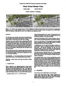
Queried Virtual Shadow Maps Markus Giegl∗ ∗ Vienna

Michael Wimmer∗

University of Technology

Figure 1: Left: shadow map reparametrization techniques (lightspace perspective shadow maps is used here) alone cannot guarantee subpixel accuracy (leading to perspective aliasing in the lower right corner and projection aliasing on the slope in the middle of the scene), even with a 40962 shadow map. Right: Queried Virtual Shadow Maps prevent both types of undersampling artifacts.

Abstract Shadowing scenes by shadow mapping has long suffered from the fundamental problem of undersampling artifacts due to too low shadow map resolution, leading to so-called perspective and projection aliasing.

calculate the direct light shadowing of a scene. This elegant approach has just one fundamental problem: The shadow map must contain enough information to allow the visibility queries to be answered with subpixel accuracy for a given frame buffer resolution, otherwise aliasing artifacts will be visible. If this information is not contained in the shadow map, then all any algorithm can do is try to mask these artifacts, e.g. by means of filtering.

In this paper we present a new real-time shadow mapping algorithm capable of shadowing large scenes by virtually increasing the resolution of the shadow map beyond the GPU hardware limit. We start with a brute force approach that uniformly increases the resolution of the whole shadow map. We then introduce a smarter version which greatly increases runtime performance while still being GPU-friendly. The algorithm contains an easy to use performance/quality-tradeoff parameter, making it tunable to a wide range of graphics hardware. CR Categories: I.3.7 [Computer Graphics]: Three-Dimensional Graphics and Realism—Color, shading, shadowing, and texture Keywords: shadowing

1

shadow, shadow map, large environments, realtime

Introduction

Shadow mapping is a very appealing approach to employ rasterization to solve the first hit visibility problem and use this result to ∗ {giegl|wimmer}@cg.tuwien.ac.at, 1040 Vienna, Austria

Figure 2: Visualization of projection and perspective aliasing. Figure 2 visualizes the source for the two forms of shadow map aliasing: Projection aliasing is stronger, the more the texel in the shadow map is projected onto a large area of the shadow receiving surface; this is the case, the more the surface normal is perpendicular to the light direction. Perspective aliasing is stronger, the nearer the shadow receiving surface is to the eye point; this is because due to the nature of the perspective projection, the closer an object is to the eye-point the more pixels it occupies on the screen. Uniform shadow mapping does not take this into account, but uses the same density of entries everywhere, whereas shadow map reparametrization techniques (see section 2 below) globally warp the geometry that is rendered into the shadow map, so that there will be more information available near the eye point when querying the shadow map; since the transformation is global, they can however do nothing against the local effect of projection aliasing.

Figure 3: The forest scene used for testing the QVSM algorithm.

A straightforward way to increase the information contained in a uniform shadow map is to increase the resolution of the shadow map texture. This becomes impractical very fast, due to its quadratic increase in memory consumption (on current hardware the maximum supported textures size, typically 4096 × 4096, is the limiting factor, even before running out of memory). This paper presents an algorithm which runs on current graphics hardware and increases the effective shadow map resolution available to shadow the scene, while avoiding the quadratic increase in memory consumption. It does so in an adaptive manner, creating more shadow map resolution where it is needed, without the need to store information from the previous frame (making it suitable for fully dynamic scenes). It thereby can guarantee subpixel accuracy with regards to the shadow map query, getting rid of both projection and perspective aliasing. It contains an intuitive to use quality vs speed tradeoff parameter, which can be used to tune it to a wide range of graphics hardware. The algorithm is orthogonal to and can therefore be combined with other techniques, such as shadow map reparametrization; we have done so for Light Space Perspective Shadow Maps [Wimmer et al. 2004].

2

Previous work

The two most important categories of shadow algorithms are shadow volumes [Crow 1977] and shadow mapping [Williams 1978]. Most of the shadow map publications try to solve the problem of aliasing artifacts. Percentage closer filtering [Reeves et al. 1987] alleviates reprojection problems by sampling the shadow map. In Variance Shadow Maps, Donelly et al [Donnelly and Lauritzen 2006] use the variance of the depth values to further improve the shadow map sampling results. A number of papers have tried to solve the perspective aliasing coming from the perspective view frustum projection through shadow map reparametrization. Originally pioneered by Stamminger and Drettakis [Stamminger and Drettakis 2002], who try to remove perspective aliasing by subjecting the shadow map to the same perspective transform as the viewer, this idea was later refined by Martin and Tan [Martin and Tan 2004] with Trapezoidal Shadow Maps, Wimmer et al [Wimmer

et al. 2004] with Light Space Perspective Shadow Maps and Chong et al [Chong and Gortler 2004] with A Lixel for Every Pixel. However, all shadow map reparametrization methods deal only with perspective aliasing. They cannot increase the principal resolution of shadow maps, which would be necessary for example to improve projection aliasing, or in cases where the scene is simply too large for the SM resolution. Furthermore, they work well only for the case that light and view direction are orthogonal. If these directions are parallel, they have to revert to uniform shadow mapping because the shadow map parametrization runs across the whole screen, not from near to distant points. Recently Lloyd et al [Lloyd et al. 2006] have studied the use of more than one shadow map applied to the sides or slices of the view frustum together with reparametrization techniques intensively, with interesting results; all these approaches can however only deal with perspective aliasing, but can do nothing to alleviate projection aliasing. The work presented in this paper aims to increase the resolution of shadow maps regardless of the view frustum orientation or whether the artifacts come from perspective or projection aliasing. Aila and Laine [Aila and Laine 2004] and Johnson et al [Johnson et al. 2005] elegantly bypass the aliasing problem altogether but depend on hardware extensions for realtime performance which are not currently available. Another approach to solve the aliasing problem are adaptive shadow maps [Fernando et al. 2001] (see also section 6 below for a comparison with Queried Virtual Shadow Maps), where shadow maps are stored in a hierarchical fashion in order to provide more resolution where it is required due to different aliasing artifacts. However, the approach requires multiple readbacks and does not map well to current graphics hardware. Lefohn [Lefohn et al. 2005] has proposed an extension that makes better use of the GPU, whereas Arvo [Arvo 2004] slices the lightview to increase the resolution of the SM. Second depth shadow mapping [Wang and Molnar 1994] can be used to reduce problems due to depth quantization and self occlusions. Brabec et al. [Brabec et al. 2002] improve uniform shadow map quality by focusing the shadow map to the intersection of the viewfrustrum with the scene. An excellent overview of shadow mapping and shadow algorithms in general can also be found in M¨oller and Haines’ Real-Time Rendering book [M¨oller and Haines 2002], as well as in [Hasenfratz et al. 2003].

3

Virtual Tiled Shadow Mapping

1. In a first pass, render the scene as described above, but into a 4 component 32bit floating point render target. In the pixel shader, store the unmodified eye-space z-coordinate into the α-component. This component forms the Eye-Space Depth Buffer (however for simplicity, we refer to the whole 4 component target as the Eye-Space Depth Buffer). The color of each pixel in the object when lit by this light (ignoring shadowing) is written to the RGB channels.

We first present Virtual Tiled Shadow Mapping. This is a bruteforce approach for increasing the resolution of the shadow map beyond the maximum texture size supported by the hardware. The basic algorithm is as follows: 1. Allocate the biggest shadow map texture supported by the GPU. For example 4096 × 4096.

2. For each shadow map tile

2. Partition the shadow map along the shadow map x- and y-axis into n × n (e.g. 16 × 16) equally-sized tiles (each tile using the full shadow map texture resolution of e.g. 4096x4096 texels, i.e. the effective resolution of the full shadow map in this example is (16 ∗ 4096) × (16 ∗ 4096) = 65536 × 65536).

(a) Render a shadow map into the shadow map texture as with Multi-Pass Shadow Mapping. (b) Instead of rendering the geometry for the whole scene again, render a full-screen quad with the Eye-Space Depth Buffer bound as a texture.

For each tile

(c) In the pixel shader for each fragment, look up the eyespace depth of the fragment in the Eye-Space Depth Buffer’s alpha-channel and unproject it into world space (see below). Using the unprojected fragment, calculate the shadowing term. Then modulate the already-shaded RGB value from the Eye-Space Depth Buffer with the shadowing term.

(a) Render a shadow map into the shadow map texture (using culling to the light frustum of the tile and overwriting the shadow map for the previous tile). (b) Use it immediately to shadow (modulate) the part of the scene which is covered by the current shadow map tile. There are two ways to implement the loop over the tiles: multi-pass shadowing and deferred shadowing.

3.1

Multi-Pass Shadowing

One way to apply successive shadow map tiles to the scene is by multi-pass rendering. In the first pass, the scene is rendered normally (with full shading and depth-writes enabled), with the first shadow map tile applied to it. For each subsequent shadow map tile, the scene is rendered again, but only shadow mapping using the relevant tile is applied to the frame buffer. Pixels falling outside the shadow map tile are suppressed. Depth writes and shading are disabled and the depth comparison function is set to EQUAL in those passes (depending on driver support, it can make sense to substitute LESSEQUAL for EQUAL).

3.2

Deferred Shadowing

Multi-pass shadowing, although easy to implement, comes with a significant performance overhead of rendering the whole scene several times. To speed up the application of the shadow map tiles to the scene, we use a variation of deferred shading we call “deferred shadowing” where the shadowing is done using a linear depth buffer of the scene instead of re-rasterizing the scene geometry and the information needed to do the next shadowing pass, i.e., the next shadow map tile, is created on the fly between the passes. The scene is first rendered to a texture that stores eye-space depth, called the Eye-Space Depth Buffer. Each subsequent tiled shadowing pass can then read this texture and calculate the world-space position of the visible surface at each pixel using the screen coordinates and the depth stored in the Eye-Space Depth Buffer. The worldspace position is then shadowed using the shadow map tile as before. Note that storing the unmodified eye-space z-coordinate in the Eye-Space Depth Buffer guarantees that the shadow map lookup produces the same results as if the original scene objects were used for shadow mapping. This is important because any other method of obtaining the z-value, e.g., using window-space z-coordinates (which is highly non-linear) or a fixed-precision w-buffer (if it were still supported on current hardware) would inevitably lead to image artifacts. In detail this works as follows:

(d) The resulting shaded and possibly shadowed fragment is then written to the frame buffer. The pixel shader operations in the individual passes are quite straightforward, with the exception of the unproject operation. Unlike a standard viewport unprojection, which transforms from window (xw , yw , zw )-coordinates to eyespace (xe , ye , ze )-coordinates, this operation has to deduce eye-space (xe , ye , ze ) from (xw , yw ) (given as texture coordinates, i.e. running from 0 to 1) and ze . This can be done using the following matrix transform:

  1 xe ax   ye  = z e ·  0 ze 0 

0

− baxx

1 ay

b − ayy

0

1

  2   0 · 0

0 2 0

   1 xw −1  ·  yw  1 1 (1)

where the parameters ax , ay , bx , by in the first matrix should be taken from the projection matrix P supplied to the graphics API: 

ax  0  P= 0 0

0 ay 0 0

bx by ... 1

 0 0   ...  0

See figure 5 for a comparison between Multipass and Deferred Shadowing.

4 4.1

Queried Virtual Shadow Mapping Smart Refinement Preferred

Virtual Tiled SMing is a brute force approach, which makes its practical applicability limited, due to the quadratic increase in the number of SM-tiles which need to be generated to increase the SM resolution by one SM-texture extent. What we would like to do instead is to adaptively refine the shadow map only where necessary: near the eye-point, and in regions with high projection aliasing. We would like to refine to a high level (n ≥ 16, i.e. ≥ 256 SM-tiles), but

(a) 40962 conventional SM

(b) 32 × 32 20482 QVSM

Figure 4: Conventional shadow mapping using LiSPSM exhibits undersampling artifacts on the trees in the foreground. The image on the right was created using Queried Virtual Shadow Maps.

Figure 5: Performance comparison of Multi-pass and Deferred Virtual Tiled Shadow Mapping: 10,000 objs, 1,6 Mtris, 4 × 4 SM-tiles on a GeForce 6600GT with 256MB, Pentium4 2.4GHz (1GB).

do it fast enough so it can be done each frame, and without breaking the GPU friendliness of the algorithm. One hypothetical way to do this is as follows. Do not shadow the scene directly, but write the results of the shadowing passes into an extra 1 × f loat texture the size of the frame buffer (“shadow result texture”). Then refine the shadow map in quad-tree fashion: First, shadow the whole shadow result texture with a single shadow map tile; then split the tile into 2 × 2 subtiles, and shadow the shadow result texture with each subtile, noting how much the increase of the effective shadow map resolution improves the shadow result texture in each tile. If the improvement achieved by the refinement is small enough, stop processing this tile further. If not, split this tile again into 2×2 subtiles, and so on. Compared to the brute force approach, this would lead to a greatly reduced number of required shadow map tiles. Unfortunately the GPU is very limited in its ability to execute such “smart” algorithms efficiently, especially those using even moderately complex data structures, such as quadtrees. Therefore we need to move the decision whether to further refine a shadow map tile to the CPU. The only straightforward way to pass the necessary information to the CPU would be reading back the whole shadow result texture after each refinement step and counting the changed pixels, which would be prohibitively expensive.

4.2

Queried Refinement: GPU Friendly & Smart

Instead, we have come up with a novel use of the GPU Occlusion Query mechanism, which counts the number of fragments emitted from the pixel shader. Occlusion queries were introduced to support image-space bounding volume visibility tests, and have seen

mainstream support by graphics hardware vendors for some time now. We use the mechanism for another purpose: when applying a shadow map subtile to the shadow result texture, we instruct the pixel shader to only produce a fragment if the resulting shadow value differs from the previous refinement step (this can easily be done by accessing the previous shadow result texture in the shader). The number of produced fragments η, which is identical to the number of changed pixels in the shadow result texture, is found by bracketing the application of each shadow map tile with an Occlusion Query. The CPU can then decide whether to further refine a tile by comparing the value returned by its corresponding occlusion query with a threshold value ηmin : if a number of pixels larger than ηmin have changed, the tile is split into 4 subtiles, otherwise the refinement for this tile stops. In addition we use the maximum number of tiles allowed per shadow map axis, ξmax , as a second refinement termination criterion. Thus, the decision whether or not to refine a shadow map tile can be made without any frame buffer readback, which allows the whole algorithm to produce larger effective shadow map resolutions in real time.

5

Jump Optimizations

Using the maximum SM texture size supported in hardware for the virtual shadow map texture is, in general, not the best choice. This comes from the fact that the minimum number of Virtual Shadow Maps that need to be filled is 1 + 4 = 5 (the initial shadow map plus one refinement step). The following two optimizations use this observation, to speed up rendering by increasing the SM texture size instead of splitting the SM:

5.1

Maximum Refinement Jump

This optimization makes use of the maximum tile refinement criterion ξmax , the maximum allowed number of tiles per shadow map axis. Before splitting a tile (of size s), we first test whether the maximum virtual shadow map resolution ξmax ·s could also be reached in one step by switching to a larger shadow map texture (i.e., a higher shadow map resolution) instead of splitting the tile. With ξ as the current tile refinement level, we make the jump if ξmax · s ≤ smax · ξ . Since we know that we will reach the maximum user defined virtual shadow map resolution for this tile and therefore will not refine this tile further, we turn off querying for the shadowing step.

the resolution is high enough. The efficiency of this mechanism allows us to perform the complete refinement procedure for each frame. This is in contrast to adaptive shadow maps, which have to cache the recently used shadow tiles for best performance - an approach which is not well suited to dynamic scenes (see the large performance drop for this case in [Lefohn et al. 2005], even though the test scene consists only of a single tree on a small quad). This also means that we do not need persistent video memory for cached tiles.

7

Results

(a) 40962 conventional SM

(b) 32 × 32 20482 QVSM

Figure 9: Performance comparison between Virtual Tiled and Queried Virtual SMing along path in forest test scene.

Figure 6: Strong projection aliasing (a) is greatly reduced by QVSM (b).

5.2

Opportunity Jump

The Opportunity Jump optimization uses a heuristic criterion to predict the future development of η (the number of pixels in the shadow result texture that changed through the last refinement step). If the prediction is that η will become smaller than ηmin within a “jump distance” (number of refinement steps) smax s , then we again do not refine the tile, but increase the shadow map texture size instead. We assume the η decreases at least by a factor fη in each refinement step in the vicinity of ηmin ; fη is a constant factor, which can be set by the user according to his quality requirements (see Results section below for a discussion of meaningful values for fη ).
smax We make the jump, if η · fη s ≤ ηmin . We again turn off querying for the shadowing step and stop any further refinement because, in the unlikely case that the tile does not reach the intended resolution, it would be disproportionally expensive to split the tile further, because we would have to use 4 shadow maps with s = smax (which would be too costly, since the premise is that we do not use s = smax for the SM-tiles from the start because of the cost of generating several smax × smax shadow maps).

6

Comparison with Adaptive Shadow Maps

Our algorithm is similar in spirit to “Adaptive shadow maps” [Fernando et al. 2001], and its GPU-based implementation, “Dynamic Adaptive Shadow Maps on Graphics Hardware” [Lefohn et al. 2005], in that it also uses a quadtree scheme to refine the shadow map (which is a more or less obvious choice). However, instead of trying to predict the required shadow map resolution for each camera pixel, we simply stop the refinement when we discover that

Figure 10: Performance comparison along path in forest test scene for several values for QVSM threshold parameter ηmin . Figure 3 depicts the test scene used for this paper. It has a large number of high frequency shadow casters (branches), which exhibit self shadowing as well as receiving shadows in an irregular manner by being far from being able to be well approximated by a shadow receiving plane. It also quite naturally leads to the eye-point being potentially very near to a shadow receiver in the form of low hanging branches or the trunk of a tree therefore making it harder to hide shadow mapping artifacts. In addition the hilly structure of the ground gives rise to projection aliasing. Unless otherwise noted, all results were created on a ATI Radeon X1900XTX with 512 MB of RAM and a Pentium4 3.4 GHz (2 GB RAM). Figure 9 shows frame time curves from a forest scene with 5 × 106 triangles rendered into a 1024 × 1024 frame buffer. The uppermost curve depicts brute force Virtual Tiled SMing, using 16 × 16 40962 shadow maps; QVSM 1 & QVSM 2 show Queried Virtual

(a) 40962 conventional SM

(b) 32 × 32 20482 QVSM

Figure 7: Quality comparison in forest test scene, rendered to 10242 frame buffer. Screenshot taken along path whose frame times are depicted in figure 9. The effective SM resolution applied to the scene on the right is 65, 5362 , 256 times larger than the SM on the left.

(a) 40962 uniform

(b) 40962 LiSPSM

(c) 20482 32 × 32 tiled

(d) 20482 32 × 32 queried

(e) 20482 32 × 32 queried + Jump Optimization

Figure 8: Comparison of the different techniques using a 512 × 512 frame buffer, 32 × 32 tiles maximum refinement and a 20482 shadow map texture (framerates can be seen in the upper right corner).

SMs with 20482 SM-tiles, 32 × 32 maximum refinement and jump optimizations to 40962 using ηmin = 2500 and ηmin = 0 respectively. The SM-curve finally gives the frame times for conventional SMing using the maximum 40962 shadow map texture currently supported in hardware (leading to greatly reduced shadow quality). LiSPSM [Wimmer et al. 2004] was active for all SM renderings. One can see that for ηmin = 0, i.e. the exact same shadowing quality, Queried Virtual SMs are more than 4 times faster than brute force Virtual Tiled SMing; for ηmin = 2500, which still gives excellent shadow quality, Queried Virtual SMs are nearly 15 times faster. The effective Virtual SM resolution used to shadow the scene is 32 × 2048 = 65536, as compared to 4096 for conventional SMing. Figure 7 shows a screenshot along the path, comparing the visual quality of conventional SMing and QVSMing. The frame times for several values of ηmin (the minimal number of pixels that need to change in a SM-tile refinement step for the tile to be refined further) along the same forest path are shown in figure 10. One can see that the frame times fluctuate more, the smaller ηmin becomes. This is due to the fact that a smaller ηmin makes the algorithm more sensitive towards changes in the scene (eye position, light direction etc), leading to more fluctuation in the

number of created SM-tiles. Figure 11 compares frame times for jump optimizations with fη = 41 . One can see that Opportunity Jumping has, in general, the greater effect. What one can also see from the curve is, that Opportunity Jumping also has a very beneficial influence on the maximum frame times, in that it cuts the frame time spikes, contributing to a smoother framerate. Having observed the behavior of η in the vicinity of ηmin , fη should be chosen to lie between fη = 21 to 18 . fη = 12 is a very conservative assumption, while fη = 18 is rather aggressive and can lead to some minor artifacts when a tile gets not refined to the desired quality; fη = 14 in general is a good compromise in practice. Figure 4 shows typical undersampling artifacts on the trees in the foreground, despite using LiSPSM. QVSM (depicted on the right) shadows the scene subpixel accurate, using 19 SM-tiles (17×20482 and 2 × 40962 ; the latter coming from optimization jumps) giving an effective SM resolution of 65, 5362 . Figure 6 shows strong projection aliasing on the right due to self shadowing. QVSM on the left removes the projection aliasing nearly completely; note that the high precision of the resulting shadow reveals the nature of the un-

thereof) are best observed in motion, http://www.cg.tuwien.ac.at/research/vr/vsm, find some demonstration videos.

we refer you to where you can

A non-scientific version of this paper was published as an article in ShaderX 5 ([Giegl and Wimmer 2007]) from the ShaderX book series; an executable and sourcecode samples can be found on the CD-ROM accompanying the book.

7.1

Figure 11: Performance comparison along path in forest test scene for QVSM Jump Optimzations.

derlying geometry by showing its triangular nature - one can see that the terrain of the scene is much coarser than the trees. The number of SM-tiles generated by the algorithm depends on the choice of ξmax , ηmin and smax and the size of the frame buffer. For quad-splitting of the SM-tiles the number of SM-tiles generated by the algorithm is 1 + 4 · k + l jump−opt , i.e. {1, 5, 9, 13, 17, }˙ + l jump−opt , where l jump−opt is the number of tiles generated by jump optimizations. In practice we found that for our test scene and frame buffer size, a typical case would be k = 4 and l jump−opt = 2 leading to 19 SM-tiles. Note that having 6 SM-tiles is a lower bound in practice, since the necessary initial refinement step from 1 to 4 SM-tiles already leads to the generation of 5 SM-tiles overall; if this is followed by a jump optimization refinement, then we arrive at 5 + 1 = 6 SM-tiles (having less SM-tiles would mean that brute force refinement into 2 × 2 SM-tiles would be the better choice). In practice the initial refinement step typically is followed by at least one further refinement step and a jump optimization refinement, leading to (k = 2,l jump−opt = 1) 10 SM-tiles overall. Figure 8 shows a comparison between different shadow mapping approaches and maximum refinement level ξmax . One can see that sample redistribution methods, represented here by LiSPSM, cannot sufficiently increase the effective shadow map resolution for this view direction. For the refinement parameter smax , we found that for an NVidia GeForce 6600GT with 256MB of RAM, 1024 × 1024 shadow map textures together with smax = 2048 proved to be efficient, whereas for an ATI Radeon 1900XTX with 512MB of RAM, using 2048 × 2048 with smax = 4096 proved to be a good choice (both graphics cards support a maximum texture resolution of 4096 × 4096). Figure 5 shows a performance comparison of Multi-pass and Deferred Virtual Tiled Shadow Mapping. One can see that for scenes which have a high transformation load, deferred shadowing gives the expected near-constant frame time. One problem that could arise in practice would be visible SM-tile boundaries in the resulting shadow due to precision issues. We did not observe such problems in our implementation, but should this problem arise, it would be very easy to fix, by simply making the SM-tiles overlap by a slight amount. Overlapping the SM-tiles leads to no artifacts, since the shadowing result does not need to be combined with the existing shadow result texture value, but overwrites previous results. In addition higher refined SM-tiles will be generated later than lower refined ones so there is also not even a potential reduction in quality in the small overlap area. Since

shadow

mapping

and

its

artifacts

(or

absence

Extensions and Optimizations

The following list some further optimizations that can be applied to the algorithm together with some results: 1. Instead of always splitting each SM-tile into 2 × 2 subtiles (quad-splitting), one can also split it along each SM-axis alternatingly (binary-splitting). Theoretically this would allow the algorithm to better adapt itself to scenarios, where the required SM resolution differs between the two SM-axes. We have implemented this extension and have observed that frame times were, in general, higher than with quad-splitting. An analysis of the created SM tiles shows, that the problem is twofold: First, in many cases there is not enough difference in required SM-resolution along each SM-axis; this means that in the end binary-splitting does a quad-split - but it costs 2 + 2 × 2 = 6 tile generations (first split the tile into 2 subtiles along one axis, then split the 2 subtiles into 2 sub-subtiles each), instead of just 2 × 2 = 4 if we do the quad-split immediately. Second, binary-splitting only gives information about the refinement status along one SM-axis in each refinement step; so even if this is not necessary the algorithm in many cases has to do “one more split”, to make sure that the tile resolution is adequate along both SM-axis. In addition, binarysplitting is harder to combine with jump optimizations efficiently, again due to the fact that in each refinement step only information about a single SM-axis is available. We conclude that the cost of binary-splitting outweighs its benefits for practical applications. 2. Another idea would be to not split into 2 × 2, but into nsub × nsub (nsub = 3, 4, . . .) subtiles in each refinement step. We have included this in our algorithm, but, again, this lead to worse frame times in all test scenes. This is because the number of generated SM-tiles becomes extremely large, even if only one tile is refined twice (which is typically the case simply due to perspective aliasing near the eye-point): Even for 3 × 3 splitting, this already leads to 1 + 2 × (3 × 3) = 19 tiles (the initial tile, a subtile and sub-subtile), compared to 9 tiles (1 + 2 × 4) for nsub = 2. n

instead of the 3. Using the relative metric ηrel < pixels−changed−in−tile n pixels−in−tile absolute ηabs < n pixels−changed−in−tile could be a better choice for deciding whether to further refine a shadow map tile. The problem here is to get n pixels−in−tile : (a) One possible way would be to reapply the shadow map tile to the Eye-Space Depth Buffer (without shadow map lookups, of course), again bracketed with an OcclusionQuery, but always emitting a fragment in the pixel shader if it lies within the current tile. The result of the OcclusionQuery would then be n pixels−in−tile .We have tried this and unfortunately it the practical cost of this operation was so high, that it outweighs any potential benefit. See “Hardware Extension” below for a potential future better way to get ηrel .

(b) A less accurate but faster method would be to calculate the number of screen-space pixels in the projection of the shadow map tile onto the ground plane of the scene (trapezoid clipped to screen-space coordinates), and use this as an approximation for n pixels−in−tile . It would of course depend on the characteristics of the scene whether this approximation works well or not.

improve the efficiency of the algorithm even further and allow for other smart algorithms that combine GPU power with CPU versatility.

4. Another approach to deferred shadowing would be to write the xyz-coordinates of each point into a float render target (RT), using multiple-RT (MRT) functionality to write the color to a second RT: We chose not to do so, since even modern graphics cards often only support MRTs having the same bit depth; this would have meant that we would have to use two 4 × f loat RTs. Since the transformation given under 1 achieves the same result with using only one linear depth entry which can be stored conveniently in the alpha-channel of just one 4 × f loat RT, we chose this approach to implement deferred shadowing.

This research was supported by the EU in the scope of the GameTools Project (www.gametools.org) (IST-2-004363).

Acknowledgements

References A ILA , T., AND L AINE , S. 2004. Alias-free shadow maps. In Proc. Eurographics Symposium on Rendering 2004, 161–166. A RVO , J. 2004. Tiled shadow maps. In Proc. Computer Graphics International 2004, 240–247. B RABEC , S., A NNEN , T., AND S EIDEL , H.-P. 2002. Practical shadow mapping. Journal of Graphics Tools 7, 4, 9–18.

8

Hardware Extension

We use the hardware occlusion query mechanism as a counter to efficiently pass back information from the GPU to the CPU. This mechanism is like a tiny loophole, since only one value can be passed back per rendering pass, and increasing the counter is linked to emitting a color value from the pixel shader (which, fortunately, in our case is what we want to do anyway). We are sure that many more smart, adaptive algorithms could be combined with fast GPU rendering if this GPU functionality would be extended to include several registers like the occlusion query fragment counter, which could e.g. be incremented/decremented (possibly by an arbitrary amount), and which would support atomic min/max operations. Since these operations are independent of the order of execution (with the exception of overflows in the case of decrement/subtraction), they would be compatible with the highly parallel vector processor design of modern GPUs. With just one additional counter register, one could, for instance, count the total number of pixels corresponding to the current shadow map tile in addition to the number of pixels that have changed in the last refinement step, allowing us to employ different refinement metrics. With 4 additional registers with min/max support one could find the screen-space bounding box around the area influenced by a shadow map tile, reducing the number of pixels that need to be touched when applying a shadow map tile to the scene.

9

Conclusion

We have presented a novel approach to increase the effective resolution of a shadow map, without incurring the respective memory cost and bypassing maximum texture size limits, by introducing Virtual Tiled Shadow Maps. Starting with this brute force approach, we have shown that it can be made faster by an order of magnitude by employing the GPU’s occlusion query mechanism to get back information about the effect of a SM-tile refinement step to the CPU. This information in turn can be used by the CPU to guide the refinement process. The refinement metric is directly correlated to the number of pixels that changed in the scene due to the SM-tile refinement, allowing the algorithm to reduce or even remove perspective and projection aliasing. We have also proposed a hardware extension that should integrate well with existing hardware architectures, which could be used to

C HONG , H., AND G ORTLER , S. J. 2004. A lixel for every pixel. In Proceedings of Eurographics Symposium on Rendering 2004. C ROW, F. C. 1977. Shadow algorithms for computer graphics. Computer Graphics (Proc. ACM SIGGRAPH 77) 11, 2, 242–248. D ONNELLY, W., AND L AURITZEN , A. 2006. Variance shadow maps. In SI3D ’06: Proceedings of the 2006 symposium on Interactive 3D graphics and games, ACM Press, New York, NY, USA, 161–165. F ERNANDO , R., F ERNANDEZ , S., BALA , K., AND G REENBERG , D. P. 2001. Adaptive shadow maps. In Proc. ACM SIGGRAPH 2001, 387– 390. G IEGL , M., AND W IMMER , M. 2007. Queried virtual shadow maps. In ShaderX 5 - Advanced Rendering Techniques, Charles River Media, 249– 262. H ASENFRATZ , J.-M., L APIERRE , M., H OLZSCHUCH , N., AND S ILLION , F. 2003. A survey of real-time soft shadows algorithms. In Eurographics State-of-the-Art Reports. J OHNSON , G. S., L EE , J., B URNS , C. A., AND M ARK , W. R. 2005. The irregular z-buffer: Hardware acceleration for irregular data structures. ACM Trans. Graph. 24, 4, 1462–1482. L EFOHN , A., S ENGUPTA , S., K NISS , J. M., S TRZODKA , R., AND OWENS , J. D. 2005. Dynamic adaptive shadow maps on graphics hardware. In ACM SIGGRAPH 2005 Conference Abstracts and Applications. L LOYD , B., T UFT, D., YOON , S., AND M ANOCHA , D. 2006. Warping and partitioning for low error shadow maps. In Proceedings of the Eurographics Symposium on Rendering 2006, Eurographics Association, 215–226. M ARTIN , T., AND TAN , T.-S. 2004. Anti-aliasing and continuity with trapezoidal shadow maps. In Proc. Eurographics Symposium on Rendering 2004, 153–160. ¨ M OLLER , T., AND H AINES , E. 2002. Real-Time Rendering, Second Edition. A. K. Peters Limited. R EEVES , W. T., S ALESIN , D. H., AND C OOK , R. L. 1987. Rendering antialiased shadows with depth maps. Computer Graphics (Proc. ACM SIGGRAPH 87) 21, 4, 283–291. S TAMMINGER , M., AND D RETTAKIS , G. 2002. Perspective shadow maps. ACM Transactions on Graphics 21, 3, 557–562. WANG , Y., AND M OLNAR , S. 1994. Second-depth shadow mapping. Tech. Rep. TR94-019, University of North Carolina at Chapel Hill. W ILLIAMS , L. 1978. Casting curved shadows on curved surfaces. Computer Graphics (Proc. ACM SIGGRAPH 78) 12, 3, 270–274. W IMMER , M., S CHERZER , D., AND P URGATHOFER , W. 2004. Light space perspective shadow maps. In Proc. Eurographics Symposium on Rendering 2004, 143–151.