CEMA’10 conference, Athens
1
Training of Perceptron Neural Network Using Piecewise Linear Activation Function Maria P. Barbarosou1 and Nicholas G. Maratos2 1
M. P. Barbarosou is with the Technological Educational Institute of Piraeus, 250 Thivon and P. Ralli Ave., GR 12244, Egaleo, Greece, and also with the Hellenic Air-Force Academy, Dekelia Air Force Base, GR 1010, Tatoi, Greece, Fax:+302105450962, E-mail:
[email protected]. 2 N.G. Maratos is with the School of Electrical and Computer Engineering, National Technical University of Athens, 9 Iroon Polytechniou St., GR 15773, Athens, Greece, Fax:+302107722281, E-mail:
[email protected].
Abstract A new Perceptron training algorithm is presented, which employs the piecewise linear activation function and the sum of squared differences error function over the entire training set. The most commonly used activation functions are continuously differentiable such as the logistic sigmoid function, the hyperbolic-tangent and the arctangent. The differentiable activation functions allow gradient-based optimization algorithms to be applied to the minimization of the error. This algorithm is based on the following approach: the activation function is approximated by its linearization near the current point, hence the error function becomes quadratic and the corresponding constraint quadratic program is solved by an active set method. The performance of the new algorithm was compared with recently reported methods. Numerical results indicate that the proposed algorithm is more efficient in terms of both, its convergence properties and the residual value of the error function.
The activation function is a key factor in the NN structure [1]. The most fuzzy applications use a piecewise linear function (PLF) [2] for activation of neurons, because of its easy handling from their limited computational resources. NNs that use PLFs as activation function is known as piecewise linear NNs (PWL NNs). These cannot be trained by a gradient based optimization method because the lack of continuous derivatives. Hence several training algorithms of PWL NNs have been developed. For example the algorithm presented in [3] is used to NNs that employs the absolute value as activation function. In addition, in [4] is proposed a basis exchange algorithm. In this paper a new algorithm for training a PWL NN is proposed. The main stage of the method is the modification of the training problem to a quadratic programming. This process is briefly described in Section 2. The main steps of the algorithm are presented in Section 3. Section 4 contains numerical results. The paper is concluded in Section 5.
1. Introduction
2. Modification of Perceptron training to a constrained quadratic optimization problem
Neural network (NN) models are of board interest to researchers in the recent years, as its applications have flooded many areas.
A graphical representation of a single hidden layer Perceptron with a single output is shown in Figure 1. The hidden layer consists of n neurons.
CEMA’10 conference, Athens
2 Hence the output of the i th neuron,
yip , corresponding to the input of the p
pth training data x , is computed as: N p p y i f wij x j ri , j 1
1 , for i [1, , n] (2)
where n is the number of neurons, x jp is the j th element of the N -dim vector
x p , that is x p [ x1p , , x jp , x Np ] , ri the input bias of the i th neuron and wij Figure 1. Graphical depiction of a single hidden layer Peceptron. In Fig. 1 each neuron passes its input which is the weighted sum of the inputs of the network plus the input bias term, through its activation function f and presents the result to its output. The proposed method adopts the 1-dim piecewise linear function (PLF) as activation of neurons: yL L f : R [ L L] , f ( y, L) y y L (1) L y L
where L 1 , its threshold. Obviously, it is nondefferential and bounded between -1 and 1. Its graph is given in Fig. 2. It has three linear pieces which are locally differentiable and two corners. This form of the activation function may be viewed as an approximation to a nonlinear amplifier. 1 0.5 f
[ wi1,, wiN ] , (2) is written equivalently
as: yip f wi x p ri , 1 for i [1, , n] . The output of the network, z p , corresponding to the x p , is the weighted linear combination of the outputs of the neurons plus the output bias: n
p
n
z i f wi x ri , 1 i yip p
i 1
i 1
(3)
where is the output bias and i the weight connecting the i th neuron to the output layer. For every given training sample, let the p th one, the output of the network,
z p , differs from the target (desired) value, t p , by (t p z p ) . The purpose of the proposed method is to determine the coefficients wij , i , ri , and in such a way that the summed over all training samples squared error, between the actual and the target output, to be minimized. Hence the total error is 2 1 M selected to be E t p z p which 2 p 1
1.5
0
-0.5
since (3) becomes:
-1 -1.5 -3
the weight connecting the j th input to the i th neuron. By considering wi
-2
-1
0 y
1
2
3
Figure 2. 1-dim PLF bounded between -1 and 1.
E ( , r ,W , )
n 1 M p t ωi f wi x p ri , 1 2 p 1 i 1
2
(4)
CEMA’10 conference, Athens
3
where M is the number of training samples, r is the vector of input bias, that is r [r1,, rn ] , W is the n N matrix of the weights connecting the inputs to the neurons that is ,, N W [ wij ]ij11, , n and is the vector of
weights connecting the outputs of neurons and the output layer of the network, that is [1,, n ] . The following property of the PLF is an easy consequence of its definition given by (1) : af ( y, L) f (ay, a L), a R (5) Take into account (5), (4) becomes: E ( , r ,W , )
2 n 1 m p Τ p t f ωi wi x ωi ri , ωi 2 p 1 i 1 (6) To simplify the formula (6), the following transformation is applied: i i , bi i wi , qi i ri , i 1,..., n (7)
Hence the error function (6) is written: Eˆ ( , q, B, )
2 n (8) 1 m p p t f bi x qi , i 2 p 1 i 1 where [ 1, , n ] , B [b1, , bn ] and q [q1,, qn ] . So the training of NN whose layout is pictured in Figure 1, is modified to the following optimization problem with inequalities constraints:
, q, B,
min Eˆ , q, B, : i 0, i 1,..., n (9)
The basic idea of the proposed approach to carry out the optimization process for the problem (9) is the following: At each algorithm iteration and i, p the PWF in problem (9) is approximated by its linearization at the current point. In doing so the problem (9) is modified to a constrained quadratic optimization problem. It is remarked that, to be valid the linearization has to be restricted within the linear piece of the PWF where its
current value belongs. The validity of the linearization, is assured by setting extra constrains. The resulting quadratic problem is solved via an active set method [5]. The original weights and bias of NN can be obtained by applying the inverse of the transformation (7) on the solution.
3. Overview of the algorithm The outline of the proposed algorithm is as follows: Initialization Input: 1) {( x1, t1),( x M , t M )} , the training set, 2) n : the number of neurons, 3) : the threshold for stopping criterion, def
4) u o o , q o , B o , o , the initial point such that bio x p qio io , {i, p} . k iteration k Step 1. Let u k , q k , B k , k be the current point. Compute f bik x p qik , ik , {i, p} . Step 2. Modify the problem (9) to the corresponding quadratic substituting i, p the PLF for its linearization and setting the proper extra constraints, so that the linearizations to be valid. Step 3. Apply the active set quadratic programming algorithm. Firstly, determine
the feasible descent direction, d * . If
d*
the algorithm ends, otherwise
determine the maximum step length a , in this direction, for point u k 1 u k a d * to be feasible. Step 4. Set k k 1 and go back to Step 1. k
(For some {i, p} at the new point u the PLF attains a corner of its graph. In these cases the linearization consider the other linear piece. As a result both the objective function and the extra constraints of the quadratic problem change at each iteration of the algorithm).
[6] provides a detailed description of both the modification process and the relative algorithm.
CEMA’10 conference, Athens
4
4. Simulation Results
4.2 2-dim Exclusive OR problem
Two benchmark problems were selected from [7]. The simulation results confirm the effectiveness of the algorithm in terms of both accuracy and speed. The algorithm was developed using Matlab.
In this example a two neurons NN is trained to output a 1, when its input is (0,0) or (1,1), and a 0, when its input is (0,1) or (1,0). The new algorithm run 50 times using each time different random starting weights and bias in (0, 1) . All times the algorithm was reaching the termination after 10 iterations and the
4.1 1-dim Function approximation The desired function is the following: 2
2 x 2 x g ( x) 0.5 sin 0.5 sin 10 10 As in [7], it was used 20 ( x, f ( x)) samples with x in (0, 1) randomly chosen, as the training set of two neurons NN. The new algorithm run 50 times using each time different random starting weights and bias in (0, 1) . All times the algorithm was reaching the termination after 4 iterations and the SSE final sum squared error 20
( g ( x p ) z p )2
was 6 104 . These are
p 1
5. Conclusion A new training algorithm for a single layer NN with a single layer output is introduced in this work. Making use of PLF as activation of neurons, it modifies the training problem to a constrained quadratic optimization problem. Numerical results confirm its effectiveness compared to other algorithms.
References
better performances than most in [7]. Furthermore, the algorithm is tested to approximate g over a larger domain. So, the algorithm used 20 random samples within (0, 9) , as the training set of 3 neurons NN and is tested for 50 different random starting weights and bias, in (0, 1) . The final SSE fluctuated between 1.9 104 and 2.3 102 after 19 and 39 iterations correspondingly. In Figure 1 it is shown the approximation of g from the output of NN with the best performance. 1.2 NN approximation Desired function and training samples
1
[1] A. Ngaopitakaul and A. Kunakorn “Selection of proper activation functions in backpropagation neural networks algorithm for transformer internal fault locations”, International Journal of Computer and Network Security (IJCNS), vol. 1, 2009, pp. 47-55. [2] W. Eppler, “Piecewise linear networks (PLN) for process control, Proceedings of the 2001 IEEE Systems, Man, and Cybernetics Conference, 2001. [3] J. Lin and R. Unbehauen, “Canonical piecewise-linear networks”, IEEE Trans. On Neural Networks, vol.6, 1995,pp. 43-50. [4] E. F. Gad, et al., “A new Algorithm for learning in piecewise-linear neural network”, Neural Networks, vol. 13, 2000, pp. 485-505. [5] D. G. Luenberger, “Linear and Nonlinear Programming”, Addison Wesley Publishing Company, Canada, 1989.
0.8
g
0.6
[6] Μ. Π. Μπαρμπαρόζοσ, “Νέα αναλογικά νεσρωνικά δίκησα και νέες μέθοδοι εκπαίδεσζης νεσρωνικών δικηύων», Διδακηορική Διαηριβή, ΕΜΠ, 2005.
0.4 0.2 0 -0.2 0
final SSE was 2.5 105 . These are by far better performances than most in [7].
1
2
3
4
5
6
7
8
x
Figure 3. The output of NN after training with the new algorithm.
9
[7] A. Bortoletti, et al. “A new class of quasiNewtonian methods for optimal learning in MLPnetworks”, IEEE Trans. On Neural Networks, vol. 14, 2003, pp. 263-273.