Robust Neural Network Training Using Partial Gradient Probing Milos Manic
Bogdan Wilamowski
Department of Computer Science University of Idaho 800 Park, Blvd. Boise, ID 83712, USA
College of Engineering University of Idaho 800 Park, Blvd. Boise, ID 83712, USA
misko@i)ieee.org
[email protected]
Abstract - Proposed algorithm features fast and robust convergence for one bidden layer neural networks. Search for weights is done only io the input layer i.e. on compressed network. Only forward propagation is performed with second layer trained automatically with Pseudo-Inversion training, for all patterns at once. Last layer training is also modified to handle non-linear problems, not presented here. Through iterations gradient is randomly probed towards each weight set dimension. The algorithm further features serious of modifcations, such as adaptive network parameters that resolve problems like total error fluctuations, slow convergence, etc. For testing of this algorithm one of most popular benchmark tests - parity problems were chosen. Final version of the proposed algorithm typically provides a solution for various tested parity problems in less than ten iterations, regardless of initial weight set. Performance of the algorithm on parity problems is tested and illustrated by figures.
solution towards robustness in terms of activation function derivative modification. Still, no universal solution towards robust and fast training algorithm has been found. The proposed algorithm features fast and robust convergence, achieved through adaptiveness of neural network parameters (learning constant, network gain, and search radius). This way algorithm typically provides a solution for various tested parity problems in less than 10 iterations. Search for weights is done only in the input layer i.e. not all weights participate in gradient calculation. Algorithm performs only forward propagation with second layer trained automatically with Pseudo-Inversion training for all patterns at once. In each iteration gradient is randomly probed towards each weight set dimension. Algorithm is further modified to alleviate occasional unwanted algorithm behavior. Those modifications automatize search for most adequate parameters (adaptive search). This way problems such ase slow convergence, fluctuations in gradient search, flat spots, local minima, or sensitivity to initial choice of network parameters, are resolved The rest of the paper is organized as following. Second section discusses weight space reduction and 2"d layer automatized training. Third section explains steps of proposed algorithm, and is followed by gradient calculation explanation. The fourth section illustrates test examples. The fifth section concludes this paper with directives for future work. Last,sixth section contains references used in this paper.
I. INTRODUCTION The proposed algorithm draws its roots from two distinctive approaches in iterative search. One is iterative gradient search method characteristical for neural networks, such as error back propagation. The other approach considers flexible approximativetechniques for neighborhood search. Neighborhood search methods are iterative procedures where for each feasible solution a neighborhood for next solution is defined. Most popular of those methods are descent method, Simulated Annealing and Tabu search. Though Tabu search originates from late 1970s, first results were independently presented by [1,2]. It was further formalized by [3,4] and [5]. It is a flexible approximation technique that uses memories or tabu lists to forbid moves that might lead to recently visited, i.e. tabu solutions. Tabu lists can help to intensify the search in 'good' regions or to diversify the search toward unexplored regions by variable tabu list size. Error Back Propagation (EBP) neural networks and gradient methods generally provide very good results [6]. Though presented a breakthrough in neural network research, backpropagation algorithm has number of disadvantages, such as oscillation, slow convergence, sensitivity to network parameters, etc. Numerous researchers targeted these problems over the years. In order to smooth the process, Rumelhart et al. [7] have proposed weight adaptation, also formulated by Sejnowski and Rosenberg [SI. To speed up the process, Fahlman [9] proposed a quickprop algorithm. Wilamowski and Torvik [IO] proposed
11.
NETWORK COMPRESSION
This algorithm considers compressed neural architecture. Let us consider general 2 layer architecture of n+ I neurons, where 1" layer consists of n-neurons and last layer of single neuron (illustrated by Fig. la). The reduction of such network starts fi-om initial number of weights, that is: Isflayer+ 2"d~ayer=n * (m+ I) + 1 * n + 1 ( 1 ) where n+l is number of neurons, and m number of inputs for 1" layer neurons, m+l is because of added bias. Last layer (n+ls' neuron) is trained by Pseudo-Inversion training, reducing the number of weights to n * ( m + l ) . Furthermore, bias weights are fixed to 1 therefore not participating in training. This way, original number of weights is reduced to input weights of the 1* layer, i.e. n * m weights.
0-7803-8200-5/03/$17.00 02003 IEEE
175
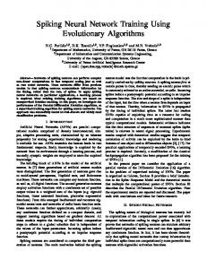
For simple 2+1 network architecture (Fig.lh) this compression reduces initial number of 9 weights to only 4 weights (weights of input connections of the fmt layer). Second layer training is automatized by Pseudo-Inversion learning rule: = ( X T X ) - I X T d(2)
w
where X’ = ( X T X ) - ’ X Tis the pseudoinverse of column matrix X,that exists even when rank is less than the dimension or when the matrix is not square. This algorihtm implements the modification of this rule known as Andersen-Wilamowski rule [11,12] to enable solving non-linear problems:
d-0
AW =(XTX)-’XT-((3)
f’
Algorithm is hrther modified to include several steps of this modified rule. This way algorithm is able to solve not only linear parity problems presented in this paper. 11.
Fig. 1. General cases of typicall one hidden layer neural network architectureused in proposed algorithm.
PROPOSED A L G O R I T H M (STEPS)
Before going into algorithm steps, certain parameters should be determined. Those are network parameters and training patterns. Network parameters are initial set ofweights, learning parameter alpha, network gain k, and search radius r. The advantage of this algorithm is its robustness with respect to these parameters, therefore all of them can be randomly chosen and algorithm will adaptively adjust them searching for fastest convergence. For tested parity problems (parity 2, 3, and 4), certain initial values for learning parameter, network gain, and search radius result in faster convergence and higher algorithm precision. Those parameters had been heuristically determined, and some of those tests are illustrated later. Tests were performed on Intel Pentium 111 lGHz, with 5 12MB SDRAM memory, Windows 2000 Pro machine.
Fig. 1. Simple three neuron case of typicall one hdden layer neural network archtecture used in proposed algonthm
weights in general case (wk wk,21, wk,22in case of 3 neuron network). For this starting weight sef gradient will be estimated in next step. Go to a next step (start with iterations).
The algorithm steps go as follows. Assign Input values. For the one hidden layer network 1. (Fig.l.a), those are n * m weights, where n is number of neurons in 1“ layer, and m is number of their input weights (1“ layer bias is fixed to 1). In case of simple 3-neuron network (Fig.lb), these are only 4 weights for inputs of first layer neurons set (wk.//, wk.21,w ~ , , ~ , Weights for the second layer neuron can be arbitrary chosen and do not influence the calculation.
4.
Start
iterations.
First
calculate
the
gradient.
Gradient is numerically calculated through gradient probing around the weight set from previous step. Such quasi-gradient is calculated in following way. Each of n * m “changeable” weights (4 in case of 3-neuron architecture), is adaptively reproduced, one at the time. Therefore, n * m cycles are performed (again in 3-neuron case, 4 cycles). In each cycle, only one of those n * m weights gets changed. The rest of the weight set is being kept the same. Now one feed-forward pass through the whole network is performed, same as in 2”dstep. The output of each cycle is the total error. This total error for is stored for later gradient each cycle ( E l , E2,..., E,,,) evaluation. Gradient in k+l”’ iteration is calculated according to following formula in vector form (4) where w,epk,llis
2. Initial Pass. One pass through the network is done. This means net, output, and finally total error (TE) is calculated for all patterns. This is done through forward calculation through the first layer, for each pattern, for all patterns. Now Pseudo inversion takes charge of training of last layer weights. This 2”d layer hypersonic training is done for all patterns at once. Once signals are propagated through the 1“ layer (for all patterns), then the 2”d layer can be efficiently trained. The outcome of this step is the initial total error EO
weight reproduced from weight wkn,in iteration k, for input i and neuronj. E,epk,m is the total error calculated for set of
~ , weights from 3d step where instead of w ~ ,reproduced
3. Assign input values for next iteration. These are total error E, and the same weight set from the la step n * m
weight w
176
~ was~used. ~
~
,
~
100). This step was introduced after unwanted behavior (stuck in local minima, flat spot/slow convergence problems), has been detected. Related behavior has been illustrated in details in section with experimental results.
gradk :
(7) Wk+I =
4.1. Adaptive reproduction of weights goes as follows. Weights are randomly changed in certain radius. The initial radius is specified at the beginning of the algorithm. Algorithm then adapts the radius value after each iteration. This adaptiveness helps algorithm to accelerate through flat spot areas and override eventual local minima problems.
,."XI
7. End of this iteration. Start a new iteration (go to Initial Pass (2ndstep). Keep doing this until the criterion for the error is satisfied.
Now the new set of weights is calculated based on the estimated gradient and set of "changeable" weights. New set of weights is calculated based on previous formula:
5.
W,,, = W ,- a * grad
k ,
8.
(5)
Interpretation of learning constant alpha is the following. Learning constant alpha multiplies all "changeable" weights by the same number, so practically accelerates the process jumping over couple of steps that would do the same. Alpha is experimentally kept in interval [OS, 1001. If it gets smaller, learning is slowed down too much ("changeable" weights decreased 10 times if alpha=0.1). This means alpha is not initialized in each iteration, it rather keeps changing to accommodate the learning process. Sometimes algorithm stays for 4-8 iterations with the similar total error. Learning constant alpha as well as other adaptive parameters do not change sooner in order to avoid fluctuations. Once the better set of weights is found, algorithm goes rapidly towards the good gradient. Adaptivity of learning constant is very importan< and performance of the algorithm significantly deteriorates without this improvement.
or in vector form (6):
wk+I,II
wk,ll
wk+l,21
wk,21
... Wk+l,ml
w,+,=..,...
... '%,m1
- ......
wk+l,ln
Wk.1"
wk+1,2n
wk,2n
a*
... wk+l,mn
.wL.-n
End of the Algorithm.
'."XI
111.
or in different form (7). Each A is randomly generated number within search radius. This set of weights is now ready to be used in next iteration. Go to next step where network parameters will be prepared for next iteration.
EXPERIMENTAL RESULTS
Experimental results were obtained through various parity problems. Activation function was bipolar. The effect of adaptive and network parameters (initial set ofweights, learning parameter alpha, network gain k, search radius r ) will be illustrated on following examples.
Adapt network parameters: learning parameter alpha, 6. network gain k, and search radius r. These parameters are modified depending on trend of total error (TE) change in previous 4 iterations. Gain and radius are increased if TE is within 10% change, decreased otherwise. Alpha is modified in similar fashion; however, criterion for alpha increase is monotonic TE decrease. In other words, alpha gets decreased in case of TE fluctuations or non-monotonic TE decrease. Intervals of these parameters are experimentally determined, and those are: alpha (0.5,100), gain (l,lO), and radius (0.5,
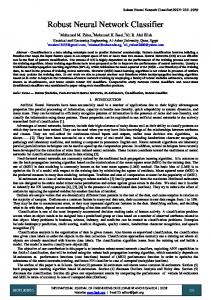
First problem was the XOR problem, tested on network architecture from Figla, with required total error of 0.5e10-8. Problems encountered and effect of introduced modifications will be illustrated. Though algorithm shows acceptable convergence rate for small gain values (around O.l), it might experience slow convergence rate (Fig.3a). For large values of gain (e10, algorithm exhibits much faster convergence (Fig.3b). Though
177
= I -
*.
, ,.
lo) leads to not only a quick but also a smooth convergence. This algorithm allows use of gain values where other algorithms such as error back propagation even fail at all. However, the more complex the parity problem, the smaller gain needs to be used to maintain the original smoothness. This was incorporated in algorithm’s adaptive logic. Algorithm allows larger random span of initial weight set with higher parity problems, while still maintaining smooth convergence. Simply, even though higher parity is more complex, algorithm has less troubles finding gradient as flat spots and local minima have less influence. For smaller parity problems larger initial weight set randomness radius can still provoke fluctuations in total error decrease through iterations. Further research includes different directions. Algorithm will be added to set of online neural network training tools, previously produced by authors and available as freeware at:httD://huskv.eneboi .uidaho.edu/nnl. Even though highly dependent on type of the problem and network architecture, mutual dependence (relationship) among
V.
REFERENCES
[I] Glover, F., “Future paths for integer programming and links to artificial intelligence”, Computers & OperationsResearch 13, pp.533-549, 1986. [2] Hansen, P., “The steepest ascent mildest descent heuristicfor combinatorial programming”, Talk presented at the Congresss on Numerical Methods in Combinatorial Optimization, Capri, 1986. [3] Glover, F., Tabu Search:prt I. ORSA Journal on Computing 1, pp. 190-206, 1989. [4] Glover, F., Tabu Search:part 11. ORSA Journal on Computing 2, pp.4-32, 1990. [5] de W m , D., Hertz, A., “Tabu search techniques: a tu1orial and an application to neuralnetworkr”,OR Spektrurn 11, pp.131-141, 1989. [6] J.M. Zurada, Artificial Neural Systems, PWS Publishing Company, St. Paul, MN, 1995. [7] Rumelhart, D.E., Hinton, G.E., and Williams, R.J., Learning internal representationby error propagation, Parallel Distributed Processing, Vol. 1, pp.318-362, MIT Press, Cambridge, MA., 1986 [8]Sejnowski T.J., Rosenberg, C.R., Parallel networks t h t learn lo pronounce English text, Complex Systems 1:145-168, 1987. [9] Fahlman S.E., “Faster-learning variations on backpropagation: An empirical study”, Proceedings of the Connectionist Models Summer School, eds. D.Touretzky, G. Hinton, and TSejnowski, Morgan Kaufmann, San Mateo, CA, 1988. [IO] Wilamowski, M., Torvik, L., "Modification ofgradient computation in the back propagalion algorifhm”, Artificial Neural Network in Engineering, Nov., St.Louis,Mssou., 1993. [I I] RJ. Schalkoff, Artificial Neural Network, McGraw-Hill, New York, 1997. [12] Wilamowski, B. M., ”Neural iietworks and F u w S w a n s ” chapters 124.1 to 124.8 in The Electronic Handbook. CRC Press 1996, pp. 1893-1914.
180