MPI+ X: task-based parallelization and dynamic load balance of finite

arXiv:1805.03949v1 [cs.MS] 9 May 2018

MPI+X: task-based parallelization and dynamic load balance of finite element assembly Marta Garcia-Gasulla, Guillaume Houzeaux, Roger Ferrer, Antoni Artigues, Victor L´opez, Jes´ us Labarta and Mariano V´azquez Barcelona Supercomputing Center, c) Jordi Girona 29, 08034 Barcelona, Spain

Abstract The main computing tasks of a finite element code(FE) for solving partial differential equations (PDE’s) are the algebraic system assembly and the iterative solver. This work focuses on the first task, in the context of a hybrid MPI+X paradigm. Although we will describe algorithms in the FE context, a similar strategy can be straightforwardly applied to other discretization methods, like the finite volume method. The matrix assembly consists of a loop over the elements of the MPI partition to compute element matrices and right-hand sides and their assemblies in the local system to each MPI partition. In a MPI+X hybrid parallelism context, X has consisted traditionally of loop parallelism using OpenMP. Several strategies have been proposed in the literature to implement this loop parallelism, like coloring or substructuring techniques to circumvent the race condition that appears when assembling the element system into the local system. The main drawback of the first technique is the decrease of the IPC due to bad spatial locality. The second technique avoids this issue but requires extensive changes in the implementation, which can be cumbersome when several element loops should be treated. We propose an alternative, based on the task parallelism of the element loop using some extensions to the OpenMP programming model. The taskification of the assembly solves both aforementioned problems. In addition, dynamic load balance will be applied using the DLB library, especially efficient in the presence of hybrid meshes, where the relative costs of the different elements is impossible to estimate a priori. This paper presents the proposed methodology, its implementation and its validation through the solution of large computational mechanics problems up to 16k cores.

1

Introduction

Although this work will focus on the first family of methods, all the strategies described here can be apThe two most intensive computing tasks of computa- plied to the second one. For each element, the system assembly consists of tional mechanics codes for unstructured meshes are the algebraic system assembly and the iterative solver two main steps: to solve it. In this paper we will focus on improving • Compute the element matrix and right-hand the performance and execution of the first task, the side. algebraic system assembly. • Assembly the element system into the local alThe algebraic system assembly consists of a loop gebraic system of each MPI partition. over elements, in the Finite Element (FE) context, and faces or cells in the Finite Volume (FV) context. The element loop is local to each MPI partition and 1

does not involve any communication. It is thus wellsuited for shared memory parallelism. In an MPI+X hybrid parallelism context, X has consisted traditionally of loop parallelism using OpenMP. However, assembling the element system into the local one involves an update of a shared variable which limits drastically the efficiency of the straightforward use of OpenMP pragmas. Several strategies have been proposed in the literature to circumvent this weakness, like the coloring or substructuring techniques to avoid the race condition appearing in the assembly of the element system into the local system. The main drawback of the first technique is the drop of the number of instructions per cycle (IPC) due to the bad spatial locality inherent to the coloring. The second technique solves this issue but requires intensive recoding, which can be cumbersome when several element loops should be treated. These techniques will be summarized in Section 3. We propose an alternative, based on the task parallelism of the element loop using an extension to the OpenMP programming model and implemented in the OmpSs model[9][4]. The taskification of the assembly that we propose solves both aforementioned problems. The technique will be described in Section 3.2.2. In addition, in the context of MPI parallelization load imbalance is an issue that can degrade the performance and does not have a straightforward solution. The main issue when load balancing an MPI application comes from the fact that the data is not shared among the different MPI processes. Consequently, application developers put a lot of effort at obtaining a well balanced data partition [23] [18] [29]. Unfortunately a well balanced partition is not always easy to obtain as we will see in Section 4. And, even, if a well balanced partition is achieved it does not imply a well balanced execution. In some cases the load can change during the execution, i.e. particles moving or a dam breaking. In this case, a runtime solution is necessary. One of the solutions proposed in the literature is to repartition the mesh during the execution to obtain a better balanced distribution [30]. This kind of solutions implies a redistribution of data and cannot be applied each timestep

because of the overhead they introduce. Moreover, they cannot react to punctual load changes or load imbalance introduced by system noise. We will apply a dynamic load balance that does not require to modify the application neither to redistribute data. Finally, in Section 5, the efficiency of the proposed taskifying strategy will be compared to classical loop parallelism with OpenMP using an element coloring strategy. In this section we will also present the performance evaluation of the load balancing library. And we will demonstrate that both mechanisms can be useful to scale a finite element code up to 16386 cores.

2

Fluid and structure dynamics

In this work we consider two different sets of partial differential equations (PDE’s), modeling incompressible flows and large deformations of structures. We will put more emphasis on the first set of equations, as the numerical modeling and system solution are more complex. Apart from the sets of equations to be solved, we will introduce as well the case examples selected to carry out the proposed optimizations. In the case of the Navier-Stokes equations we will consider the airflow in the respiratory system, while for structure mechanics, we will consider a fusion reactor.

2.1

Fluid solver

The high performance computational mechanics code used in this work is Alya [27], developed at BSC-CNS, and part of the Unified European Application Benchmark Suite (UEABS) [6]. This suite provides a set of scalable, currently relevant and publically available codes and datasets, of a size which can realistically be run on large systems, and maintained into the future. In this section, will briefly describe the CFD module of Alya and its parallelization. 2.1.1

Physical and Numerical models

The equations governing the dynamics of an incompressible fluid are the so-called incompressible 2

Navier-Stokes equations. They express the Newton’s second law for a fluid continuous medium, whose unknowns are the velocity u and the pressure p of the fluid. Two physical properties are involved, namely µ be the viscosity, and ρ the density. At the continuous level, the problem is stated as follows: find the velocity u and pressure p in a domain Ω such that they satisfy in a given time interval

work. We extract the pressure Schur complement of the pressure unknown p and solve it with the Orthomin(1) method, as detailed in [12]. The resulting algorithm is shown in Algorithm 2. In the algorithm,

Algorithm 2 Algebraic solver: Orthomin(1) method for the pressure Schur complement. 1: Solve momentum eqn Auu uk+1 = bu − Aup pk ∂u + ρ(u · ∇)u − ∇ · [2µε(u)] + ∇p = 0, (1) ρ 2: Compute Schur complement residual rk = [bp − ∂t Apu uk+1 ] − App pk ∇ · u = 0, (2) 3: Solve continuity eqn Qz = rk 4: Solve momentum eqn Auu v = Aup z together with initial and boundary conditions. The 1 5: Compute x = App z − Apu v velocity strain rate is defined as ε(u) := 2 (∇u + t 6: Compute α = (rk , x)/(x, x) ∇u ). 7: Update velocity and pressure The variational multiscale (VMS) method is ap k+1 plied to discretize this set of equations, as extensively p = pk + αz described in [15]. In addition, the velocity subgrid (4) uk+2 = uk+1 − αv scale is tracked in convection and time. This means that apart from solving for the previous unknowns u and p, an additional equation is solved to obtain the ˜ . A typical assembly for the grid scale subgrid scale u equations consists in a loop over the elements of the matrix Q is the pressure Schur complement preconditioner, computed here as an algebraic approximation mesh, as shown in Algorithm 1. of the Uzawa operator, and as explained [12]. On Algorithm 1 Assembly of a generic matrix A and the one hand, the momentum equation is solved with the GMRES method and diagonal preconditioning in vector b. steps 1 and 4 of the algorithm. On the other hand, 1: for elements e do the continuity equation is solved with the Deflated 2: Compute element matrix and RHS: Ae , be Conjugate Gradient (DCG) method [19] with linelet 3: Assemble matrix Ae into A preconditioning [25] in step 3 of the algorithm. The 4: Assemble RHS be into b deflation provides a low frequency damping across the 5: end for domain, especially very efficient for the case study considered in this work, where the geometry is elongated. The linelet preconditioner consists of a tridi2.1.2 Algebraic system solution agonal preconditioner applied in the normal direction After the assembly step, the following monolithic al- to the boundary layer mesh near the walls. gebraic system for the grid scale unknowns, velocity At each time step, this system is solved until conu and pressure p, is obtained: vergence is achieved. Convergence is necessary be     cause the original equation is non-linear (the convecAuu Aup u bu = . (3) tive term makes matrix Auu depend on u itself). For Apu App p bp any information concerning the parallel solution sysThis system can be solved directly using a Krylov tem 3 on distributed memory supercomputers, see solver and efficient preconditioner [24]. However, [16, 12]. Only a brief description will be given herein an algebraic-split approach is used instead in this in Section 3.1. 3

2.1.3

Subgrid scale

core flow. Figure 1 shows some details of the mesh, and in particular the prisms in the boundary layer. Once the velocity u and pressure p are obtained on We will see in Section 4.1 how the presence of difthe nodes of the mesh, the velocity subgrid scale vecferent types of elements makes difficult the control tor is obtained through a general equation of the form of the load balance when using the mesh partitioner METIS. −1 ˜ = τ (Ru + bu˜ ) , u (5) where τ is the so-called stabilization diagonal matrix and R is the residual rectangular matrix, as the subgrid scale is obtained element-wise and not node-wise. ˜ and thus Equation Both τ and R may depend on u ˜ 5 can be non-linear. Note finally that in practice, u is obtained via a simple loop over the elements of the mesh and the system of the equation does not need to be explicitly formed. 2.1.4

Solution strategy

In practice, the iterations of the Orthomin(1) iterative solver to solve for the pressure Schur complement are coupled to the non-linearity iterations of the Navier-Stokes equations, which include not only the convective term but also the subgrid scale. The resulting workflow is shown in Algorithm 3. The workflow consists of three main computational kernels. The assembly which carries out operations on the elements of the mesh in order to construct the algebraic system; the algebraic solver, that is the algorithm for the pressure Schur complement, which consists in solving twice the momentum equation and once the continuity equation; finally, the subgrid scale calculation which is computed on the elements of the mesh and thus involves a loop over the elements. 2.1.5

Figure 1: Respiratory system, details of the mesh.

2.2

Structure solver

The structure mechanics solver is extensively described in [8]. For the sake of completeness, we will only briefly describe the set of equations to be solved. 2.2.1

Physical and Numerical models

The equation of balance of momentum with respect to the reference configuration can be written as

Case example: respiratory system

ρ0

For the evaluation of the different techniques described in the following sections we will consider the case of the respiratory system, similar to that described in [7]. The mesh is hybrid and composed of 17.7 million elements: prisms to resolve accurately the boundary layer; tetrahedra in the core flow; pyramids to enable the transition from prism quadrilateral faces to tetrahedra. This kind of mesh is quite representative in fluid dynamics, as most of the fluid problems of interest involve boundary layers and a

∂2u − ∇ 0 · P = b0 , ∂t2

(6)

where ρ0 is the mass density (with respect to the reference volume) and ∇0 · is the divergence operator with respect to the reference configuration. Tensor P and vector b0 stand for the first Piola-Kirchhoff stress and the distributed body force on the undeformed body, respectively. Equation 6 must be supplied with initial and boundary conditions. To discretize this equation, the Galerkin method is used in space and the Newmark method [5] in time. 4

Algorithm 3 Solution strategy for solving Navier-Stokes equations. 1: for time steps do 2: while until convergence do 3: Assemble global matrices and RHS of Equation 3 using Algorithm 1 4: Solve momentum equation with GMRES, step 1 of Algorithm 2 5: Solve continuity equation with DCG, step 3 of Algorithm 2 6: Solve momentum equation with GMRES, step 4 of Algorithm 2 7: Compute subgrid scale using Equation 5 8: end while 9: end for A Newton-Raphson method is used to solve the lin- 3 Parallelization of Algebraic earized system. For each time step, and until conSystem Assembly vergence, one has to assemble the algebraic system using Algorithm 1 (where A is the Jacobian and b For the sake of completeness, this section describes is the residual of the equation) and then solve the briefly the classical parallelization techniques of a ficorresponding algebraic system for the displacement nite element assembly in an HPC environment. unknown. According to the characteristic of this system, the GMRES or the DCG methods are considered. 3.1 Distributed Memory Paralleliza-

tion Using MPI 2.2.2

In the finite element context, two options are available when defining a distributed memory parallelization, which we refer to as partial-row and full-row methods [20]. In the finite difference context or in the finite volume context using a cell centered discretization scheme, the second method is generally considered, as it emerges naturally. In the finite element community, the partial-row method is quite natural when partitioning the original element set (mesh) into disjoint subsets of elements (subdomains). In this case, nodes belonging to several subdomains (interface nodes) are duplicated. As the matrix coefficients come from element integrations, the coefficients of the edges involving interface nodes are never fully assembled. The resulting local (to each MPI subdomain) matrices are therefore square matrices. However, if one considers iterative solvers to solve the resulting algebraic system (which is the case in this work), the main operation consists of Sparse Matrix-Vector Products (SpMV) y = Ax. Thus, there is no need for obtaining these global coefficients, as the result y can be computed locally on each subdomain and then assembled later on inter-

Case example: Iter

The mesh is a slice of a torus shaped chamber, representing the center part of a nuclear fusion reactor called the vacuum vessel. In Figure 2 we can see the representation of the mesh made of 31.5 million hexahedra, prisms, pyramids and tetrahedra elements.

Figure 2: Iter, mesh.

5

3.2

face nodes using MPI send and receive messages (by associativity of the multiplication operation). The full-row approach consists in assigning nodes exclusively to one subdomain. This strategy leads to local rectangular matrices, and these matrices are fully assembled blocks of rows of the global matrix. Two options are thus possible. A first option in which the global matrix coefficients of the interface nodes can be obtained by summing up the contributions coming from neighboring subdomains, thus obtaining full rows. This can be achieved through MPI communications.

3.2.1

Shared Memory Parallelization Using OpenMP Loop parallelism

During the last decade, the predominance of general purpose clusters have obliged parallel code designers to devise distributed memory techniques, mainly based on MPI, as briefly described in last subsection. Then, while the number of CPUs has been multiplied, the number of subdomains has been increasing. The side effect is the increase of communication which limits the strong scalability, and the increase of number of MPI subdomains, which limits the weak scalability. Nowadays, supercomputers offer a great variety of architectures, with many cores on nodes (e.g. Xeon Phi). Thus, shared memory parallelism is gaining more and more attention as a it offers more flexibility to parallel programming. This parallelism has traditionally been based on OpenMP, a programming model enabling a straightforward parallelization through simple pragmas. Finite element assembly consists in computing element matrices and right-hand sides (A(e) and b(e) ) for each element e, and assembling them into the local matrices and RHS of each MPI process, namely A and b, as shown in Algorithm 1. This assembly has been treated using mainly three techniques, as illustrated in Figure 3. All of these techniques are based on loop parallelism, each of them offering different advantages and drawbacks. The main issue is the race condition appearing in the assembly scattering the element arrays A(e) and b(e) into the local ones, A and b. The first method consists in avoiding the race condition using ATOMIC pragmas to protect these shared variables (Figure 3 (left)). The cost of the ATOMIC limits the scalability of the assembly. This strategy is shown in Algorithm 4. In the context of vectorization, the element coloring technique has been proposed [10, 21]. By coloring elements such that elements with the same color do not share nodes, no ATOMIC is required to protect A and b. The main drawback of this method is that any spatial locality of data is lost which implies a low IPC (instructions per cycle). In the performance evaluation based in hardware counters included in Section 5,

A second option in which the mesh is partitioned into disjoint subsets of nodes. The full rows of the matrix are thus obtained by assigning all the necessary elements to the subdomains in order to get all the element contributions. In this case, interface elements must be duplicated (halo elements), leading to duplication of the work during the assembly process on these halo elements. As far as SpMV is concerned, MPI communications are performed before the product on the multiplicand x. The advantage of the partial-row approach is that the load balance of the assembly can be controlled, in principle, when partitioning the mesh. With partitioners like METIS [17], the number of elements per subdomain can in addition be constrained with the minimization of the interface sizes. The main drawback is that while balancing the number of elements per subdomain, one loses control on the number of nodes, which dictates the balance of SpMV. On the other hand, the presence of halo elements in the fullrow approach limits the scalability, due to the duplicated work on them and to the lack of control on the number of elements per subdomain. When considering hybrid meshes, an additional difficulty arises, as one has to estimate the relative weights of the different element types in order to balance the total weight per subdomain, as we will show in Section 5. Thus, no matter if full-row or partial-row is ultimately chosen, load imbalance will occur before starting the simulation. In this work, the partial-row approach is considered and described in [27], while load imbalance will be treated in Section 4. 6

Figure 3: Shared memory parallelism techniques using OpenMP. (a) ATOMIC pragma. (b) Element coloring. (c) Local partitioning. we will show that the loss in IPC is up to 100% due to the ATOMIC pragma, while it is of 50% using the coloring technique respect using a pure MPI version. This strategy is shown in Algorithm 5. To unify the terminology with other techniques, we define a subAlgorithm 4 Matrix Assembly without coloring in domain as a set of elements of the same color, and each MPI partition nsubd the total number of subdomains, that is the 1: !$OMP PARALLEL DO & total number of colors. 2: !$OMP SCHEDULE (DYNAMIC,Chunk_Size) & To circumvent these two inconveniences, local par3: !$OMP PRIVATE (...) & titioning techniques (in each MPI partition indepen4: !$OMP SHARED (...) dently) have been proposed [2, 26]. Here, classical 5: for elements e do partitioners like METIS or Space Filling Curve based 6: Compute element matrix and RHS: Ae , be partitioners can be used. Elements are assigned 7: !$OMP ATOMIC to subdomains, and subdomains are unconnected 8: Assemble matrix Ae into A through separators (layer of elements) such that ele9: !$OMP ATOMIC ments of neighboring subdomains do not share nodes. 10: Assemble RHS be into b By assigning elements to a subdomain, the loop over 11: end for elements is substituted by the parallelization of the loop over subdomains. This techniques guarantees spatial locality and avoids the race condition. However, this force us to treat the separators differently (e.g. by re-decomposition) and makes its implemen7

Algorithm 5 Matrix assembly with coloring in each MPI partition 1: Partition local mesh in nsubd subdomains using a coloring strategy 2: for isubd = 1, nsubd do 3: !$OMP PARALLEL DO & 4: !$OMP SCHEDULE (DYNAMIC,Chunk_Size) & 5: !$OMP PRIVATE (...) & 6: !$OMP SHARED (...) 7: for elements e in isubd do 8: Compute element matrix and RHS: Ae , be 9: Assemble matrix Ae into A 10: Assemble RHS be into b 11: end for 12: !$OMP END PARALLEL DO 13: end for

3.2.2

Task parallelism

It is possible to implement another strategy by forgoing the loop parallelism approaches shown above and using a task parallelism approach instead. As of OpenMP 3.0 a new tasking model was introduced which allows the OpenMP programmer to parallelize a set of problems with irregular parallelism. When a thread of the OpenMP program encounters a TASK construct it creates a task which is then run by one of the threads of the parallel region. In principle the order, i.e. the schedule, in which the tasks are run is not determined by the creation order. OpenMP 4.0 allows constraining the schedule by adding the possibility of defining dependences between tasks. This way the OpenMP programmer can use a data-flow style for irregular parallelism. While intuitive, the dependency approach based on input and output dependences is too strict for a problem like the finite element assembly. It forces the runtime to determine a particular order (necessarily influenced by the task creation order) that fulfills the dependences when executing the tasks. The research in the OmpSs programming model [28] led to the proposal of a new kind of dependency between tasks called COMMUTATIVE. This new dependency kind means that two tasks cannot be run concurrently if they refer to the same data object but does not impose any other restriction in the particular order in which such exclusive execution happens. This kind of dependency is suitable for our problem as, in principle, we do not really care which subdomain is processed first as long as two subdomains that share a border are not processed concurrently. A further complication exists, though, for the current dependency support in OpenMP 4.0 implies that the number of dependences is statically defined at compile time. This is inconvenient as each subdomain may have a variable number of neighbors. To address this we use the multidependences extensions in which each task may have a variable number of dependences [28]. In this way, the tasking parallelization is possible by first computing the adjacency list of each subdomain. Figure 4 depicts this idea, where the subdomain 3 has 5 neighbors (including itself).

tation more complex. The algorithm is shown in Algorithm 6. We can observe the similitude between Algorithm 6 Matrix assembly with local partitioning in each MPI partition 1: Partition local mesh in nsubd subdomains using METIS 2: for isubd = 1, nsubd do 3: !$OMP PARALLEL DO & 4: !$OMP SCHEDULE (DYNAMIC,Chunk_Size) & 5: !$OMP PRIVATE (...) & 6: !$OMP SHARED (...) 7: for elements e in isubd do 8: Compute element matrix and RHS: Ae , be 9: Assemble matrix Ae into A 10: Assemble RHS be into b 11: end for 12: !$OMP END PARALLEL DO 13: end for 14: Treat separators

the loops of the coloring and local partitioning techniques. The differences are in the way the subdomains are obtained (coloring vs METIS) and the existence of separators in the local partitioning technique. 8

Given that adjacency list, it is then possible to use Algorithm 7 Matrix assembly with commutative a COMMUTATIVE multidependence on the neighbors. multidependences in each MPI partition This causes the runtime to run as many subdomains 1: Partition local mesh in nsubd subdomains of size as possible in parallel that do not share any node. Chunk Size 2: Store connectivity graph of subdomains in structure subd 3: for isubd = 1, nsubd do 4: nneig = SIZE(subd(isubd)%lneig) 5: !$OMP TASK & 6: !$OMP COMMUTATIVE 7: ([subd(subd%lneig(i)), i=1,nneig]) & 8: !$OMP PRIORITY (nneig) & 9: !$OMP PRIVATE (...) & 10: !$OMP SHARED (subd, ...) 11: for Elements e in isubd do 12: Compute element matrix and RHS: Ae , be Assemble matrix Ae into A Figure 4: Task parallelism using multidependences: 13: 14: Assemble RHS be into b neighbors of subdomain 3 (including itself). 15: end for 16: !$OMP END TASK As subdomains are processed, less of them will re17: end for main and the parallelism available will decrease. It is possible to get higher concurrency levels if, of all the 18: !$OMP TASKWAIT non-neighboring subdomains, we first process those with a bigger number of neighbors: intuitively this potentially can free more subdomains that are not neighbors. To this end, we prioritize subdomains with a higher neighbor count. We can achieve this using the PRIORITY clause. Algorithm 7 shows the final task parallelization. For each subdomain: we create a task (step 5); then we declare a commutative dependency with all its neighbors (step 7); we prioritize tasks with a higher number of neighbors (step 8). These tasks are created by a single thread inside of a parallel region (not shown in the listing) and the thread will not proceed until all of them have been run by itself or other threads of the team (step 18).

that it works on distributed memory, thus, each MPI process will work on the data in its subdomain. This fact makes the mesh partitioning crucial, as it will determine the load balance of the execution. Although there are techniques to redistribute or repartition the mesh during the execution, these are expensive as they require to move data between processes and to modify the code the code to repartition when necessary. The mesh partitioning software provides, in general, load balancing features which necessarily are based on optimizing a metric. As we discussed in the introduction, the main computational tasks of a CFD and structure mechanics codes are the algebraic system assembly and the iterative solver. 4 Dynamic Load Balancing We want to obtain a partition that ensures load balance in the matrix assembly. But in hybrid meshes 4.1 MPI Load Imbalance the number of elements might not be a good metric As we explained in Section 3.1, using an MPI paral- to measure the load balance, as their relative weights lelization implies partitioning the original mesh into in constructing the matrix may be different. n subdomains. The essential characteristic of MPI is In this paper we focus on the assembly phase, 9

Load Balance =

0,8 0,7 0,6 0,5 0,4 0,3

Assembly T Theoretical -LB Assembly -W Weighted LB Assembly -M Measured Assembly Subscale -T Measured SGS Subscale - W

0,2 0,1 0

Useful CPU time = Total CPU time n X

16

32

64 128 256 # MPI partitions

512

1024

Figure 5: Load Balance for the Respiratory system.

ti

i=1

1

n · maxni=1 ti

0,9

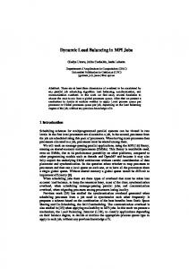
Let us define we the weight of element e and nie the number of elements of partition i. We define two theoretical load balance (LB) measures: the nonweighted load balance which is the ratio of the average number of elements to the maximum number of elements, as well as the weighted load balance, which represents the same including the weights given to METIS (that is what METIS load balances). We also introduce the measured load balance obtained by measuring the elapsed time (timei ) of each MPI task in the assembly or subgrid scale loop and dividing the average by the maximum of the elapsed times. Pn Pni ( i MPI e e we )/nMPI , Pni maxi ( e e we ) Pn ( i MPI nie )/nMPI Theo. non-weighted LB = , maxi nie Pn ( i MPI timei )/nMPI Measured LB = . maxi (timei )

Load Imbalance (Avg/Max)

=

1 0,9 Load Balance (Avg/Max)

for this reason we want to obtain a partition that achieves a well balanced distribution of elements among the different MPI processes. In a hybrid mesh, the computational loads of different elements are not the same. As a intuitive guess, we will assign as a weight to each element the number of Gauss points used in the matrix assembly. We define Load Balance as the percentage of time that the computational resources are doing useful computation:

0,8 0,7 0,6 0,5 0,4 0,3 Theoretical LB Weighted LB Measured LB

0,2 0,1 0 16

32

64 128 256 # MPI partitions

512

1024

Figure 6: Load Balance for the Iter simulation.

and the Measured LB has been measured from an execution of the simulation and averaged over 10 time steps. We first observe that METIS provides a fairly good load balance based on the heuristic provided for both meshes (weighted LB), even though an imbalance up to 14% is observed for 512 partitions in the respiratory system. We can say that the theoretical load Figures 5 and 6 show the load balance measured for balance achieved by METIS depends on the mesh the two use cases presented in the previous section. structure and the number of partitions, more partiThe X axis represents the number of MPI partitions tions tend to higher load imbalances, we can observe used for each simulation. The different values have this specially in the case of the respiratory system. been computed using the formulas presented above But if we compare this theoretical result with Theo. weighted LB

=

10

the measured one, we can see a significant difference. In practice the load imbalance increases with the number of partitions, specially for the Respiratory system, for both the assembly and for the subgrid scale element loops (which are quite similar). We conclude that the number of Gauss points is absolutely not a good measure of the work per element. Indeed, the measured load balance follows the non-weighted load balance. On the contrary, the load balance of the Iter simulation seems to follow the weighted load balance. This means that the same heuristic cannot be used to obtain a well balanced partition of different problems.

(a) Partitioning.

Finally, let us take a look at typical partitions and traces. Figures 7(a) and 8(a) shows some statistics of the partitions for the fluid and solid problems using 256 CPUs. The nodes are placed at the centers of gravity of the MPI subdomains, while the edges represent neighboring relations. We observe that in the case of the respiratory system, METIS happens parti(b) Trace. tions some MPI subdomains into non connected parts (identified by the arrow). We also observe that one Figure 7: Respiratory system simulaiton on 256 subdomain has much more elements than the others CPUs. (identified with an arrow in the middle figure). This is the subdomain located at front of the face (see Figure 1), which is exclusively composed of tetrahedra. 4.2 DLB library Tetrahedra have less Gauss points and thus METIS Load imbalance is a concern that has been targeted admits more elements than in average. since the beginning of parallel programming. In the The associated traces are shown in Figures 7(b) literature, we can see that it has been attacked from and 8(b). In the case of the Respirartory system, very different points of view (data partition, data rewe can easily identify the subdomains responsible for distribution, resource migration, etc.). In this case we are using METIS to partition the the load imbalance, near the bottom of the trace. These are the subdomains mentioned previously, in mesh and obtain a balanced distribution among MPI the front face region. This is because the element tasks. But as we have seen in the previous section, weight based on the Gauss points given to METIS is the actual load balance obtained is far from optimal. There are several reasons for this, the geometry of the not a good metric. mesh and the weight of the elements given to METIS. Additionally, the algorithm or the physics (or both In the case of the Iter simulation, we can observe that we have some subdomains with much less work together) could produce very strong work imbalance than others. Once more, this indicates that the by increasing the computing needs locally (i.e. parweights based on Gauss points is not a good heuris- ticle concentrations [14], solid mechanics fracture, tic for load, although it affects much less the load shock in compressible flows, etc.) For these reasons, we opt for a dynamic approach applied at runtime, balance than for the fluid simulation. 11

on the same node that it is still doing computation.

(a) Partitioning.

Figure 9: (Left) Unbalanced MPI+OpenMP application. (Right) Unbalanced MPI+OpenMP application balanced with DLB.

(b) Trace.

Figure 8: Iter simulation on 256 CPUs.

with no need for an a-priori imbalance analysis. In this work we will use DLB [11] (Dynamic Load Balancing Library). The DLB library aims at balancing MPI applications using a second level of parallelism (i.e. Hybrid parallelization MPI+OpenMP). Currently, the implemented modules balance hybrid MPI + OpenMP and MPI + OmpSs applications, where MPI is the outer level of parallelism and OpenMP or OmpSs are the inner ones. An important feature of the DLB library is that a runtime interposition technique is used to intercept MPI calls. With this technique we do not need to modify the application, the DLB library is loaded dynamically when running the application to load balance the execution. The DLB library will reassign the computational resources (i.e. cores) of an MPI process waiting in an MPI blocking call, to another MPI process running

Figure 9 illustrates the load balancing process. In the example, the application is running on a node with 4 cores. Two MPI tasks are started on the same node, and each MPI task spawns 2 OpenMP threads (represented by the wavy lines). Eventually, an MPI blocking operation (in green) synchronizes the execution. Regarding the assembly process, the wavy lines represent the element loops and the MPI call represents the first MPI call in the iterative solvers (namely the initial residual of the algebraic system). On the one hand, Figure 9 (Left) shows the behavior of an unbalanced application where the excessive work of the threads running on core3 and core4 delays the execution of the MPI call. On the other side, Figure 9 (Right) shows the execution of the same application with the DLB library. We can see that when the MPI task 1 gets into the blocking call it will lend its two cores to the MPI task 2. The second MPI task will use the newly acquired cores and will be able to run with 4 threads. This will allow to finish the remaining computation faster. When the MPI task 1 gets out of the blocking call it retrieves its cores from the MPI task 2 and the execution continues with a core equipartition, until another blocking call is met. The fact that DLB relies on the shared memory to load balance the different MPI tasks means that it needs to run more than one MPI task per node. In current many-cores architectures this is the normal

12

trend The dynamic load balancing algorithm illustrated previously relies on the OpenMP parallelization. One important characteristic of this strategy is that not the whole application needs to be fully parallelized, as the second level of parallelism can be introduced only for load balancing purposes, in the main imbalanced loops of the code.

5 5.1

• 8x2: 8 MPI processes with 2 threads each. • 16x1: 16 MPI processes with 1 thread each. In this case, the shared memory level is only used for load balancing. This configuration is useful when the application is not fully parallelized with OpenMP/OmpSs and it is launched as a pure MPI application. • Pure MPI: As a reference we show the performance of the pure MPI version of the application, in this case 16 MPI processes are launched on each node.

Performance Evaluation Environment and Methodology

For each experiment we will execute different verAll the experiments presented in Section 2 have been sions, in Table 1 we present detailed summary of each executed on MareNostrum 3 supercomputer. Each data series that we will see in the charts. node of MareNostrum 3 is composed of two Intel We have divided the evaluation into four parts: Xeon processors (E5-2670), each of this two sockets • Chunk size: In this section we will study the includes 8 cores and 16 GB of main memory. In total impact of the chunk size on the performance each compute node has 16 cores with 32GB of main of the different parallelizations and when using memory. DLB. From this evaluation, we will try to find We have used the Intel MPI library version 4.1.3 the optimum chunk size, and use it for the foland as the underlying Fortran compiler Intel 13.0.1. lowing experiments. For OpenMP we have used Nanos 0.12 [4][9] with the source to source compiler Mercurium 2.0 [3]. For • Execution Time: In this evaluation we will the dynamic load balancing we have used the DLB show the performance obtained by the three library 1.3. shared memory parallelization alternatives: No We have executed the experiments on 16, 32 and 64 Coloring, Coloring, and Multidependencies, in nodes of MareNostrum 3 that correspond to 256, 512 terms of elapsed execution time. We will also and 1024 cores, respectively. For each experiment we see the impact in performance of using the dywill consider 5 different configurations of MPI pronamic load balancing mechanism. cesses and threads inside the node: • Hardware Counters: In this section we • 1x16: 1 MPI process with 16 threads, this is the demonstrate our hypothesis in the performance pure hybrid approach, where MPI is used across of each parallelization, based in the different nodes and OpenMP/OmpSs inside the shared hardware counters collected during the execumemory node. In this configuration, DLB cantion. not load balance, but we show it for complete• Scalability: Finally we will present some scalaness. bility tests of the Respiratory system simulations using up to 16K cores of MareNostrum 3. • 2x8: 2 MPI processes with 8 threads each. This is another typical configuration when running in nodes with two sockets, each MPI process is 5.2 Chunk Size Study mapped to one socket, and 8 threads are spawn In this section, we want to evaluate the impact of the on each socket. chunk size on the performance of the different par• 4x4: 4 MPI processes with 4 threads each. allelization alternatives and DLB. In OpenMP the 13

1: Different methodologies tested. Shared mem. Dynamic Algorithm parallelism load balance Loop No Alg. 4 Loop No Alg. 5 Task No Alg. 7 Loop DLB Alg. 4 Loop DLB Alg. 5 Task DLB Alg. 7 None No Alg. 1

3,5

Race condition treatment ATOMIC Coloring technique Multidependencies ATOMIC Coloring technique Multidependencies Not applicable

No coloring Coloring Multideps

3

No coloring + DLB Coloring + DLB Multideps + DLB

2,5 Time (s)

2 1,5 Pure MPI

1 0,5 6000

5000

4000

3000

2000

900

Chunk size

1000

800

700

600

500

400

300

200

90

100

80

70

60

50

40

30

20

10

0

(a) 16 Nodes (256 cores) No coloring Coloring Multideps

2 1,8

No coloring + DLB Coloring + DLB Multideps + DLB

1,6 1,4 1,2 1 0,8 Pure MPI

0,6 0,4 0,2 4000

5000

6000

3000

4000

5000

3000

2000

Chunk size

1000

900

800

700

600

500

400

300

200

100

90

80

70

60

50

40

30

20

0 10

(b) 32 Nodes (512 cores) No coloring Coloring Multideps

1 0,9

No coloring + DLB Coloring + DLB Multideps + DLB

0,8 0,7 0,6 0,5 0,4 0,3

Pure MPI

chunk size determines the number of iterations (in our test case one iteration corresponds to the computation of one element) that are executed sequentially by one thread. When using a parallel loop approach (both coloring and no coloring) the chunk size is defined using the schedule clause SHEDULE(DYNAMIC, ). In the multidependencies version the chunk is defined by the number of elements that are assigned to each subdomain. In Table 2 we summarize the number of chunks that are created in the different scenarios that we are executing, when partitioning the problem in 256, 512 and 1024 MPI partitions. As we have seen in the previous section, for a given partition the number of elements assigned to each MPI process may be different, for this reason in the table we show 3 values, the maximum number of chunks, the minimum and the average of all the MPI processes. All the experiments have been executed with 16 MPI processes per node and 1 thread per process. With this configuration, we want to evaluate the impact of the chunk duration, the amount of chunks in the queue and the impact in the malleability when using DLB. Using only one thread will avoid seeing the overhead of several threads accessing the shared structures or invalidating the memory.

Time (s)

Table Programming model MPI + OpenMP MPI + OpenMP MPI + OpenMP MPI + OpenMP MPI + OpenMP MPI + OpenMP MPI

Time (s)

Hybrid method No coloring Coloring Multideps DLB no coloring DLB coloring DLB multideps Pure MPI

0,2 0,1 2000

1000

900

800

700

600

500

400

300

200

100

90

80

70

60

50

40

30

20

10

0

Respiratory system simulation In Figure 10 we Chunk size can see the execution time of the matrix assembly in (c) 64 Nodes (1024 cores) the Respiratory system simulation. The X axis represents the different chunk sizes used. Figures 10(a), Figure 10: Respiratory system, matrix assembly: 10(b) and 10(c) correspond to executions on 16, 32 chunk size impact on execution time. and 64 nodes of MareNostrum 3, respectively. 14

Chunk size 100 500 1000 2000

256 Partitions Max Min Average 2004 522 691,3 400 104 137,8 200 52 68,7 100 26 34,1

512 Partitions Max Min Average 1369 255 345,4 273 51 68,7 136 25 34,1 68 12 16,8

1024 Partitions Max Min Average 697 101 172,5 139 20 34,1 69 10 16,8 34 5 8,2

Table 2: Respiratory system: number of chunks created for the multidependences version. No coloring Coloring Multideps

No coloring + DLB Coloring + DLB Multideps + DLB

0,8 0,6 0,5 0,4

Pure MPI

Time (s)

0,7

0,3 0,2 0,1 6000

5000

4000

3000

2000

900

Chunk size

1000

800

700

600

500

400

300

200

90

100

80

70

60

50

40

30

20

10

0

(a) 16 Nodes (256 cores) No coloring Coloring Multideps

0,7 0,6

No coloring + DLB Coloring + DLB Multideps + DLB

0,5 0,4 0,3 Pure MPI

Time (s)

0,2 0,1 4000

5000

6000

3000

4000

5000

3000

2000

Chunk size

1000

900

800

700

600

500

400

300

200

100

90

80

70

60

50

40

30

20

10

0

(b) 32 Nodes (512 cores) No coloring Coloring Multideps

0,35 0,3

No coloring + DLB Coloring + DLB Multideps + DLB

0,25 0,2

Pure MPI

0,15 0,1 0,05 2000

1000

Chunk size

900

800

700

600

500

400

300

200

100

90

80

70

60

50

40

30

20

0 10

The impact of the chunk size when using DLB comes from the fact that bigger chunks imply less malleability because threads can not leave a chunk until it is finished. The Coloring version with DLB is the most affected one by big chunks, after chunks of size 200 the performance slowly degrades until it reaches the same performance as the Coloring version with DLB. This is because the parallelism of the Coloring version opens and closes for each color, and bigger chunks means fewer chunks to be distributed among the threads, and therefore, less parallelism. If there is not enough parallelism when DLB tries to spawn more threads to load balance, there is not enough work for all of them. In the case of Coloring and Multidependencies using big chunk sizes can limit the performance obtained by DLB when the number of chunks created in each MPI process is not enough to balance the load.

1 0,9

Time (s)

In the case of the execution without DLB, the No Coloring and Coloring versions are not affected by the chunk size, until reaching very small values, chunk sizes of 10 or 20. On the other hand, the Multidependencies version starts to degrade its performance at chunk sizes between 30 and 60 depending on the number of partitions. This is related to the number of chunks that are created and their commutative relationship. When using bigger chunk sizes the execution time is not affected for none of the three parallelizations.

(c) 64 Nodes (1024 cores)

Figure 11: Respiratory system, subgrid scale: chunk Figure 11 shows the execution time of the subgrid size impact on execution time. scale computation for the Respiratory system simulation, when varying the chunk size. The conclusions for this experiments are very similar to the previous ones. The limit in the chunk size is around 20, from this size the performance of the Coloring and 15

12 Pure MPI

11,5 11

6000

5000

4000

3000

2000

500

1000

100

no_coloring coloring Multideps 50

40

30

10

10

20

Multideps + LeWI no_coloring + LeWI coloring + LeWI

10,5

Chunk size

no chunk

Time (s)

13 12,5

(a) 16 Nodes (256 cores) 7 6,8 6,6 6,4 6,2 6 5,6

6000

5000

4000

3000

2000

500

1000

no_coloring coloring Multideps 50

40

10

5

30

Multideps + LeWI no_coloring + LeWI coloring + LeWI

5,2

100

5,4

Chunk size

no chunk

Pure MPI

5,8

20

Big chunk sizes, like before, affect only when running with DLB. And the worst performance with big chunks is obtained by the Coloring parallelization. We consider that a chunk size of 200 is the optimum value for all the versions and configurations. This will be the chunk size used in the experiments executed in the following sections for the respiratory simulation.

14 13,5

Time (s)

No coloring versions degrade. For very small chunks sizes the overhead of creating the tasks and scheduling them is too high. In this case, the limit chunk size is bigger because the durations of the tasks are smaller if we compare the total execution time and considering that the number of elements that are processed in the parallel loop is the same.

no chunk

6000

5000

4000

3000

2000

500

1000

100

50

40

30

20

10

Pure MPI

Time (s)

Iter simulation Figure 12 shows the execution (b) 32 Nodes (512 cores) time of the matrix assembly for the Iter simulation. 3,6 In these charts, we have adjusted the scale of the Y 3,5 3,4 axis to see some differences between the different se3,3 3,2 ries. Each chart corresponds to a number of nodes 3,1 (16, 32 and 64), while the X axis represents the dif3 2,9 ferent chunk sizes. In this case, the Coloring and No 2,8 Multideps + LeWI no_coloring no_coloring + LeWI coloring 2,7 Coloring versions are not affected by the chunk size. coloring + LeWI Multideps 2,6 This is because the duration of these chunks in this simulation is much higher than in the Respiratory Chunk size system case. The matrix assembly in solid mechanics (c) 64 Nodes (1024 cores) requires a costly calculation of the constitutive model at the Gauss points, involved in the Jacobian matrix. Figure 12: Iter, matrix assembly: chunk size impact On the other hand, the Multidependencies version on execution time. is still limited by small chunk sizes, because its limitation does not only come from the duration of the 5.3 Execution Time chunks but also from the amount of chunks in the queue and with a commutative relationship. In this section we will compare the execution times of When using DLB the use of big chunk sizes im- the matrix assembly and subgrid scale computations plies a loss of performance. The Coloring version is for the Respiratory system and matrix assembly for the most affected one, because of the synchroniza- the Iter simulations, with and without DLB, for each tions between the loops computing the different col- parallelization technique listed in Table 1. ors. The no coloring and Multidependencies are affected in a similar way. Respiratory system simulation Figure 13 shows For this simulation the optimal chunk size in all the the execution time of the matrix assembly of the Resseries is around 100. This the chunk size that we will piratory system simulation. Figures 13(a),13(b) and use for this simulation in the following experiments. 13(c) correspond to executions on 16, 32 and 64 nodes 16

No coloring No coloring + DLB Coloring Coloring + DLB Multideps Multideps + DLB

3

Time (s)

2,5 2 1,5

Pure MPI

1 0,5 0 16x16

32x8

64x4 MPIs x Threads

128x2

256x1

(a) 16 Nodes (256 cores) No coloring No coloring + DLB Coloring Coloring + DLB Multideps Multideps + DLB

1,8 1,6

Time (s)

1,4 1,2 1 0,8 Pure MPI

0,6 0,4 0,2 0 32x16

64x8

128x4 MPIs x Threads

256x2

512x1

(b) 32 Nodes (512 cores) No coloring No coloring + DLB Coloring Coloring + DLB Multideps Multideps + DLB

0,9 0,8

Time (s)

0,7 0,6 0,5 0,4 Pure MPI

0,3 0,2 0,1 0 64x16

128x8

256x4 MPIs x Threads

512x2

1024x1

(c) 64 Nodes (1024 cores)

Figure 13: Respiratory system, matrix assembly: execution time.

respectively. The X axis represents the different configurations of MPI processes and threads used in each case, while the Y axis represents the average execution time of the assembly over ten time steps. When comparing the three different implementations of the parallelization without DLB, we can see the difference in performance that they obtain. Being the No Coloring version the worst one, performing worse than the pure MPI version in all the configurations. As we already mentioned in previous sections, the problem of the No coloring technique is the use

of ATOMICS to avoid the race condition. The Coloring parallelization yields a better execution time than the No coloring one, but still far from using the pure MPI version, due to the worst data locality. Finally, the Multidependencies implementation achieves the best performance. When using a configuration filling the nodes with MPI processes and only one thread per MPI process (i.e. configurations 256x1, 512x1 and 1024x1) the execution time obtained is very close to the pure MPI version. In this case the OpenMP level is not used and we are just measuring the overhead introduced. For the other configurations the Multidependencies implementation achieves a better performance than the MPI pure version. In general the best configuration is to spawn one MPI process per socket (2 per node) and use the OpenMP parallelism within the socket with 8 threads (i.e. configurations 32x8, 64x8 and 128x8). All the versions present a worse imbalance when increasing the number of MPI processes per node (and decreasing the number of threads), because the load imbalance increases with the number of MPI processes, see Figure 5 (Left). Except in the case of just one MPI process per node and 16 threads, where the threads may access memory belonging to the other socket of the node and these data accesses are slower. When using 8, 4 or 2 MPI processes per node, each MPI process is pinned to one of the sockets of the node. Therefore, all the data accesses will be to the local memory of the socket. When looking at the executions with DLB we observe that in all the cases DLB improves the performance of the analogous execution without DLB. The only situation where DB can not be applied is when running one MPI process per node and 16 threads per MPI process because DLB needs more than one MPI process in each node to load balance. Nevertheless, in this situation DLB does not add any overhead. Although the performance of the parallelization affects DLB, in some cases, the load balance can overcome the overheads of the parallelization and obtain a better performance than the pure MPI version. For example, in Figure 13(b), when running in 64 nodes (512 cores) and 512 MPI processes with one thread per process, the performance of the Coloring version

17

is 47% slower than the pure MPI version, but when using DLB the performance of the Coloring execution is 14% faster than the pure MPI. It is interesting to see how the performance of DLB improves with the number of MPI processes on the node, being the best configuration to fill the nodes with MPI processes and only one thread for OpenMP. This can be explained because having more MPI processes gives DLB more flexibility to load balance. i.e. if we use 2 MPI processes per node configuration, the load balance can only be applied to the two MPI processes running on the same node. In all the cases the best situation is to use the commutative Multidependencies with DLB, which can represent a 37% faster execution than the pure MPI version.

No coloring No coloring + DLB Coloring Coloring + DLB Multideps Multideps + DLB

0,8 0,7

0,5 0,4

Pure MPI

Time (s)

0,6

0,3 0,2 0,1 0 16x16

32x8

64x4 MPIs x Threads

128x2

256x1

(a) 16 Nodes (256 cores) No coloring No coloring + DLB Coloring Coloring + DLB Multideps Multideps + DLB

0,45 0,4

Time (s)

0,35 0,3 Pure MPI

0,25 0,2

0,15 0,1 0,05 0 32x16

64x8

128x4 MPIs x Threads

256x2

512x1

(b) 32 Nodes (512 cores) No coloring No coloring + DLB Coloring Coloring + DLB Multideps Multideps + DLB

0,25 0,2 Time (s)

0,15 Pure MPI

Figure 14 shows the execution time of the subgrid scale calculation, for the same experiments. In this case the No Coloring version obtains a performance close to the pure MPI execution when using 1 thread per MPI process. In the subgrid scale computation, the ATOMIC clause is not necessary, as it is obtained element-wise. For this reason, the performance compared the to the pure MPI version is much better than the one obtained in the matrix assembly. Moreover, in the subgrid scale using a hybrid method with the No coloring version is the best configuration. The coloring version performs worse than the no coloring because it still presents the bad locality issue. The Multidependencies parallelization has a performance close the that of the No coloring one for a low number of threads. When increasing the number of threads to 16, the execution time is higher because all the threads accessing the shared queue of commutative tasks in the OpenMP runtime. However, it still improves the performance of the pure MPI version. When using DLB, the performance is improved in all the cases. The best configuration with DLB is to use 16 MPI processes per node and one thread per process independently of the parallelization strategy used. When using the no coloring or Multidependencies version the performance with DLB is almost constant independently of the configuration of MPI processes and threads used. This means that DLB is able to solve all the load imbalance within the node and

0,1 0,05 0 64x16

128x8

256x4 MPIs x Threads

512x2

1024x1

(c) 64 Nodes (1024 cores)

Figure 14: Respiratory system, subgrid scale: execution time. that it is independent of the configuration decided by the user. When running in 64 nodes, the version of Multidependencies with DLB and one thread per MPI process is 44% faster than the pure MPI version. Iter simulation Figure 15 shows the execution time of the matrix assembly phase for the Iter simulation. The different charts correspond to executions on 16, 32 and 64 nodes. The X axis, we can see the different configurations of MPI processes and OpenMP threads. As already noticed in Figure 5

18

No coloring No coloring + DLB Coloring Coloring + DLB Multideps Multideps + DLB

14,5 14

Time (s)

13,5

ference between the Coloring and Multidependencies is not very significant because in this simulation the amount of computation per element is higher than when solving the Respiratory system. This means that the data locality has less impact on the overall performance. The simulations executed with DLB are always faster than their analogous ones without DLB. As in the case of the fluid, the best performance is obtained when using 16 MPI processes per node and one thread per MPI process. When using DLB with Multidependencies and 16 MPI processes per node, the performance is better that the pure MPI version (around 5% improvement).

13 12,5 12 Pure MPI

11,5 11 10,5 10 16x16

32x8

64x4 MPIs x Threads

128x2

256x1

(a) 16 Nodes (256 cores) No coloring No coloring + DLB Coloring Coloring + DLB Multideps Multideps + DLB

7,5

Time (s)

7 6,5 6

5.4

Pure MPI

5,5

In this subsection, we are going to evaluate the different parallelizations (No Coloring, Coloring, and Multidependencies) based in different performance counters in order to support some of the performance explanations we have used in the previous sections. The data shown in the following charts have been obtained with Paraver from an Extrae trace of a real execution using PAPI 5.4.1 [1] [22]. We are going to see the results for both simulations the respiratory system and the iter simulation. In all the cases we have launched 256 MPI processes with one OpenMP thread per MPI process (16 MPI processes per node). This configuration is used to see the impact of the parallelization in the performance of the code but to avoid seeing the contention between the different threads, as the optimum distribution of threads per MPI process has already been discussed in the previous section.

5 32x16

64x8

128x4 MPIs x Threads

256x2

512x1

(b) 32 Nodes (512 cores) No coloring No coloring + DLB Coloring Coloring + DLB Multideps Multideps + DLB

3,6 3,5

Time (s)

3,4 3,3 3,2 3,1 3 Pure MPI

2,9 2,8 2,7 2,6 64x16

128x8

256x4 MPIs x Threads

512x2

Hardware Counters Study

1024x1

(c) 64 Nodes (1024 cores)

Figure 15: Iter, matrix assembly: execution time.

(Right), the imbalance exhibited by this simulation is not very high. Therefore, the performance improvement that we can expect with DLB will not be as high as the ones obtained in the Respiratory system simulation. Note that in this case; we have increased the scale of the X axis in order to discern better the different values.

Respiratory system simulation Figure 16 is a normalized histogram of the IPC obtained during the matrix assembly. The X axis represents the different intervals of IPC measurements, while the Y axis gives the percentage of time of each IPC range, with respect to the total CPU time spent in the matrix When comparing the performance of the different assembly. We observe that the pure MPI version had parallelizations, we can see that the No Coloring ver- an IPC between 2.1 and 2.3. When using the No sion is slower than Coloring and Multidependencies Coloring version of the parallelization the IPC went because of the ATOMIC overhead. In this case, the dif- down to 1.1. This matches the previous performance 19

Pure MPI No Coloring Coloring Multideps

To back up our conclusions on the previous charts, we have measured the total number of instructions executed during a matrix assembly and subgrid scale computation. The results obtained are shown in Figure 18(a). In these charts we can see that the number

% time

100 90 80 70 60 50 40 30 20 10 0

IPC range

Figure 16: Respiratory system, matrix assembly: IPC.

1,5E+12

results were the No Coloring version was two times slower than the pure MPI. The IPC of the Coloring version is between 1.5 and 1.7, better than the No Coloring but still far from the IPC obtained by the pure MPI version. When using the Multidependencies parallelization, the IPC is between 2 and 2.2 almost the same as the one achieved by the pure MPI version.

1,0E+12

5,0E+11

0,0E+00 # Instructions Assembly

# Instructions SGS

(a) Number of instructions

Figure 17 gives the IPC for the subgrid scale computation phase. The IPC for the pure MPI and

Pure MPI No coloring Coloring Multideps

4,0E+09

Pure MPI No Coloring Coloring Multideps

% time

100 90 80 70 60 50 40 30 20 10 0

Pure MPI No coloring Coloring Multideps

2,0E+12

3,0E+09

2,0E+09 IPc range

1,0E+09

Figure 17: Respiratory system, subgrid scale: IPC. the Multidependencies versions are the same as in the matrix assembly. The No Coloring version in this phase presents a much higher IPC because it does not need the ATOMIC clause. An IPC equivalent to the one achieved with Multidependencies is obtained. On the other hand, the Coloring parallelization has a worse IPC than the others because of the loss in data locality. But we can see that the performance loss is not as important as in the matrix assembly phase, this is because in the subgrid scale computation, the pressure over the memory is not as high as in the matrix assembly phase.

0,0E+00 # L3 Misses Assembly

# L3 Misses SGS

(b) Number of L3 cache misses

Figure 18: Respiratory system: performance counters. of instructions executed in the subgrid Scale computation is much lower than the ones necessary to compute the matrix assembly. When comparing the different parallelizations we can observe that the number of executed instructions in the different parallelizations is the same, this means that the amount

20

of computation for the different parallelizations is the same. The difference in the performance come from other sources, for example the cache misses. Figure 18(b) shows the cache misses in L3 during the execution of the matrix assembly and the subgrid scale computation. As we already said, the pressure on the memory is much higher in the matrix assembly than in the subgrid scale computation. When comparing the different parallelizations, we observe that the No coloring version has the same number of cache misses than the pure MPI version, as the execution order is the same. On the other hand, the number of cache misses in the Coloring version is much higher due to loss of data locality when computing elements that are not contiguous in memory. The Multideps version presents more cache misses than the pure MPI version but far from the number of cache misses achieved by the Coloring version.

almost the same performance as the pure MPI version. Figure 20(a) shows that the number of instructions necessary to compute the matrix assembly is the same for all the parallelizations. By looking at the L3 cache Pure MPI No coloring Coloring Multideps

1,6E+12

Pure MPI No coloring Coloring Multideps

5,0E+09 4,0E+09

1,2E+12

3,0E+09 8,0E+11

2,0E+09 4,0E+11

1,0E+09 0,0E+00

0,0E+00

# L3 Misses Assembly

# Instructions Assembly

(a) Number instructions

(b) Number misses

of

L3

cache

% Time

Figure 20: Iter, matrix assembly: Performance counIter simulation Figure 19 shows the IPC obtained ters. in the matrix assembly for the Iter simulation. As we misses for the different parallelizations (Figure 20(b), 100 Pure MPI 90 No coloring we observe the same conclusions as in the Respira80 Coloring Multideps 70 tory system simulation: the No coloring version has 60 50 the same cache misses as the pure MPI; the Color40 30 ing parallelization presents a higher number of misses 20 10 and the Multidependencies version has a worse data 0 locality than the pure MPI but far from the number IPC range of misses of the Coloring one. Figure 19: Iter, matrix assembly: IPC.

Pure MPI No coloring Coloring Multideps

3

said before, the matrix assembly of this problem has a higher computational load per element than that of the fluid problem, and this can be seen in the higher IPC in all the cases. The pure MPI version has an IPC around 3 almost during the whole phase. The No Coloring version goes down to an IPC of 2.5 but still far from dividing the IPC by two that we observed in the Respiratory system simulation. Again, this confirms that there is more computation going on, and the impact of the ATOMIC clause is not as high as in the other case. The Coloring parallelization presents an IPC of 2.7 because of the worst data locality, and the Multidependencies version obtains an IPC of 2.9 achieving

L3 miss tatio

2,5 2 1,5 1 0,5 0 Respiratory Assembly

Respiratory SGS

Iter Assembly

Figure 21: Iter, matrix assembly: L3 Miss ratio. We define the miss ratio as the number of cache misses issued for each 1000 instructions executed, computed as follows: L3M issRatio = #M issesL3∗1000 #Instructions . In Figure 21 we can see the L3 miss ratio for the different simulations and computation phases. Based in this chart we can asses that the

21

8,00

pressure in the data access is much higher in the matrix assembly of the respiratory simulation than in the other computations. In the case of the matrix assembly for the iter simulation the miss ratio is lower than for the subgrid scale computation of the respiratory simulation.

5.5

Coloring Coloring + DLB Multideps Multideps + DLB Pure MPI

Time (s)

4,00

Scalability

2,00 1,00 0,50

During this evaluation, we had the opportunity to run some strong scalability tests on MareNostrum 3 with up to 16384 cores (1024 nodes). For this, we have used the mesh multiplication strategy described in [13] to obtain a mesh of 141 million elements from the original mesh shown in Figure 1. In these experiments, we wanted to demonstrate that DLB can scale up to using thousands of cores and also that even working at the node level the use of DLB can help improving the performance significantly in this kind of executions. In these executions we have simulated the Respiratory system using the best configurations observed in the previous experiments, 16 MPI processes per node with 1 thread per process and chunks of 200 elements. The values presented are the average execution time of 10 time steps for each phase of the computation.

0,25 0,13 1024

2048

4096 # Cores

8192

16384

(a) Matrix Assembly 2,00

Coloring Coloring + DLB Multideps Multideps + DLB Pure MPI

Time (s)

1,00

0,50

0,25

0,13

0,06

Figure 22 shows the execution time of the matrix assembly and the subgrid scale. In the X axis, we can see the number of cores used to run and in the Y axis the elapsed time in seconds in a logarithmic scale. As we have seen before, the performance of the coloring version is worse than the pure MPI. On the other hand, the Multidependencies parallelization obtains the same performance as the pure MPI version independently of the number of cores used. If we look at the results obtained using DLB, we can see that the execution time is reduced significantly when running with the Coloring or the Multidependencies parallelizations, but specially with the last one. The most interesting thing is to see how the gain when using DLB is maintained independently of the number of nodes used. In particular, comparing with the pure MPI version the gain goes from 1.55 to 1.75 using 1024 and 16384 cores, respectively,

1024

2048

4096 # Cores

8192

16384

(b) Subgrid Scale

Figure 22: Respiratory system: execution time up to 16k cores. Figure 23 shows the scalability as it is usually presented by application developers, using as base case the smallest number of resources used of the same version: Scalabilityx,y =

time1024,y . timex,y

We want to show how misleading this metric can be. In this chart, the best scalability is obtained by the Coloring version without DLB. But this version

22

16,0

Scalabilty

8,0

Coloring Coloring + DLB Multideps Multideps + DLB Pure MPI

In this chart, we can observe how the performance of the DLB versions is significantly better even when running on a large number of cores, being able to obtain a speed up of 23 when using 16 times more resources.

4,0

32,0 2,0

16,0

Speed up

1,0 0,5 1024

2048

4096 # Cores

8192

16384

Scalability

8,0

4,0 2,0

(a) Matrix Assembly 16,0

8,0

Coloring Coloring + DLB Multideps Multideps + DLB Pure MPI

1,0

Coloring Coloring + DLB Multideps Multideps + DLB Pure MPI

0,5 1024

2048

4096 # Cores

8192

16384

8192

16384

(a) Matrix Assembly 4,0

32,0 2,0

16,0

1,0

Speed up

8,0

0,5 1024

2048

4096 # Cores

8192

16384

Coloring Coloring + DLB Multideps Multideps + DLB Pure MPI

4,0 2,0

(b) Subgrid Scale 1,0

Figure 23: Respiratory system: scalability up to 16k cores.

0,5 1024

2048

4096 # Cores

is the one that obtains the worst execution time. On (b) Subgrid Scale the other hand, the executions with DLB (both with Coloring and Multidependencies) has a worse scala- Figure 24: Respiratory system: speedup up to 16k bility curve, but a better execution time. cores. Figure 24 shows the speed up with respect to the pure MPI version on 1024 cores. In this case, all the versions are computed versus the same baseline scenario and are thus directly comparable: 6 Conclusions Speedupx,y =

time1024,Pure MPI . timex,y

In this paper we have presented two runtime mechanisms to improve the performance of a computational 23

dynamics code. Both approaches can be used without important modifications in the source code and are applied at runtime. We have tested both mechanisms in the solutions of two production computational mechanics problems, involving a fluid and a solid. These two problems present different performance issues. On one hand, we have presented the use of multidependences to avoid a race condition in the matrix assembly, for which we have demonstrated that the performance can be improved up to a 60% when using the multidependences approach with respect to the use of ATOMICS. We have explained using a hardware counters analysis this improvement, related to avoiding the use of ATOMICS and obtaining a better spatial locality. On the other hand, we have used a dynamic load balancing library (DLB) to improve the load balance in some phases. DLB can be used without modifying the source code and we have shown an improvement in performance of up to 50%. Moreover, we have seen that the use of DLB releases the user from choosing the better configuration for a hybrid parallel programing (i.e. distribution of MPI processes and threads). DLB can be used also in MPI pure applications, just by adding OpenMP pragmas where necessary, in this case the second level of parallelism is only used for load balancing purposes. Finally we have shown that both mechanisms can scale up to 16384 cores obtaining the best results with the multidependences and DLB versions.

References

[4] Barcelona Supercomputing Center. OmpSs Specification https://pm.bsc.es/ompssdocs/spec/. [5] Belytschko, T., Liu, W., and Moran, B. Nonlinear Finite Elements for Continua and Structures. Wiley, 2000. [6] Bull, M. UEABS: the unified european application benchmark suite, October 2013. [7] Calmet, H., Gambaruto, A., Bates, A., ´ zquez, M., Houzeaux, G., and Doorly, Va D. Large-scale CFD simulations of the transitional and turbulent regime for the large human airways during rapid inhalation. Computers in Biology and Medicine 69 (2016), 166–180. ´rusalem, A., Samaniego, C., [8] Casoni, E., Je Eguzkitza, B., Lafortune, P., Tjahjanto, ´ ez, X., Houzeaux, G., and Va ´ zquez, D., Sa M. Alya: computational solid mechanics for supercomputers. Arch. Comp. Meth. Eng. 22, 4 (2015), 557–576. ´, E., Badia, R., [9] Duran, A., Ayguade Labarta, J., Martinell, L., Martorell, X., and Planas, J. Ompss: a proposal for programming heterogeneous multi-core architectures. Parallel Processing Letters 21, 02 (2011), 173–193. [10] Farhat, C., and Crivelli, L. A general approach to nonlinear fe computations on sharedmemory multiprocessors. Comp. Meth. Appl. Mech. Eng. 72, 2 (1989), 153–171.

[1] Papi: http://icl.cs.utk.edu/papi/index. [11] Garcia, M., Corbalan, J., and Labarta, html - last accessed july 2017. J. LeWI: A Runtime Balancing Algorithm for ´ zquez, M., Nested Parallelism. In Proceedings of the In[2] Aubry, R., Houzeaux, G., Va ternational Conference on Parallel Processing and Cela, J. M. Some useful strategies for un(ICPP09) (2009). structured edge-based solvers on shared memory machines. Int. J. Num. Meth. Eng. 85, 5 (2011), ´ zquez, [12] Houzeaux, G., Aubry, R., and Va 537–561. M. Extension of fractional step techniques for [3] Barcelona Supercomputing Center. Merincompressible flows: The preconditioned orcurium: https://pm.bsc.es/mcxx - last acthomin(1) for the pressure schur complement. cessed may 2017. Comput. Fluids 44 (2011), 297–313. 24

[13] Houzeaux, G., de la Cruz, R., Owen, H., Proceedings of the International Conference on ´ zquez, M. Parallel uniform mesh multiand Va Computational Science, ICCS 2011. plication applied to a navier-stokes solver. Com[23] Pearce, R., Gokhale, M., and Amato, puters & Fluids 80 (2013), 142–151. N. M. Scaling techniques for massive scalefree graphs in distributed (external) memory. In [14] Houzeaux, G., Garcia-Gasulla, M., CaProceedings of the 2013 IEEE 27th International jas, J., Artigues, A., Olivares, E., ´ zquez, M. Dynamic load Symposium on Parallel and Distributed ProcessLabarta, J., and Va ing (Washington, DC, USA, 2013), IPDPS ’13, balance applied to particle transport in fluids. IEEE Computer Society, pp. 825–836. Int. J. Comp. Fluid Dyn. (2016), 408–418. [15] Houzeaux, G., and Principe, J. A varia- [24] Saad, Y. Iterative Methods for Sparse Linear Systems. SIAM, 2003. tional subgrid scale model for transient incompressible flows. Int. J. Comp. Fluid Dyn. 22, 3 ¨ hner, R., and Camelli, F. [25] Soto, O., Lo (2008), 135–152. A linelet preconditioner for incompressible flow solvers. Int. J. Num. Meth. Heat Fluid Flow 13, ´ zquez, M., Aubry, R., [16] Houzeaux, G., Va 1 (2003), 133–147. and Cela, J. A massively parallel fractional step solver for incompressible flows. J. Comput. ´bault, L., Petit, E., Tchiboukdjian, [26] The Phys. 228, 17 (2009), 6316–6332. M., Dinh, Q., and Jalby, W. Divide and conquer parallelization of finite element method as[17] Karypis, G., and Kumar, V. MeTis: Unsembly. In International Conference on Parallel strctured Graph Partitioning and Sparse Matrix Computing - ParCo2013 (Muncih (Germany), Ordering System, Version 2.0, 1995. 10-13 Sept. 2013), vol. 25 of Advances in Paral˘, B. Solv[18] Koroec, P., ilc, J., and Robic lel Computing, pp. 753–762. ing the mesh-partitioning problem with an ant´ zquez, M., Houzeaux, G., Koric, S., colony algorithm. Parallel Computing 30, 5 [27] Va Artigues, A., Aguado-Sierra, J., Ar´ıs, (2004), 785 – 801. Parallel and nature-inspired R., Mira, D., Calmet, H., Cucchietti, F., computational paradigms and applications. Owen, H., Taha, A., Burness, E. D., Cela, ¨ hner, R., Mut, F., Cebral, J., Aubry, [19] Lo J. M., and Valero, M. Alya: Multiphysics enR., and Houzeaux, G. Deflated precongineering simulation towards exascale. J. Comditioned conjugate gradient solvers for the put. Sci. 14 (2016), 15–27. pressure-poisson equation: Extensions and im´ , M., Chasprovements. Int. J. Num. Meth. Eng. 87 (2011), [28] Vidal, R., Casas, M., Moreto apis, D., Ferrer, R., Martorell, X., 2–14. ´, E., Labarta, J., and Valero, M. Ayguade `s, F., Roux, F., and Houzeaux, [20] Magoule Evaluating the impact of OpenMP 4.0 extenG. Parallel Scientific Computing. Computer Ensions on relevant parallel workloads. 60–72. gineering Series. ISTE-John Wiley & Sons, 2016. [29] Walshaw, C., and Cross, M. Mesh parti[21] Misra, J., and Gries, D. A constructive proof tioning: A multilevel balancing and refinement of vizing’s theorem. Inform. Process. Lett. 41, 3 algorithm. SIAM Journal on Scientific Comput(1992), 131 – 133. ing 22, 1 (2000), 63–80. [22] Moore, S., and Ralph, J. User-defined events [30] Wang, M., Ren, X., Li, C., and Li, Z. Dmrfor hardware performance monitoring. Procepar: A dynamic mesh repartitioning scheme for dia Computer Science 4 (2011), 2096 – 2104. dam break simulations in OpenFOAM. In 2016 25

17th International Conference on Parallel and Distributed Computing, Applications and Technologies (PDCAT) (Dec 2016), pp. 210–215.

26