AbstractâUpcoming 5G wireless technology will enable vari- ous new applications and is going to support a massive amount of devices per cell. In this regard ...
Multi-Cell Flow-Level Performance of Traffic-Adaptive Beamforming under Realistic Spatial Traffic Conditions Henrik Klessig, Maciej Soszka, and Gerhard Fettweis Vodafone Chair Mobile Communications Systems Dresden University of Technology, Germany Email: {henrik.klessig, maciej.soszka, fettweis}@tu-dresden.de
Abstract—Upcoming 5G wireless technology will enable various new applications and is going to support a massive amount of devices per cell. In this regard, ultra-dense small cell deployments are a means to cope with the need of extremely high data rates of several tens of Gbps and with the increasing data traffic demand. However, denser deployments may lead to more severe inter-cell interference, which is strongly connected to the actual spatial distribution of the mobile traffic demand. Traffic-adaptive beamforming using phased antenna arrays can be an attractive solution for concentrating capacity at desired traffic hot spot locations while inter-cell interference is reduced. In this paper, we propose a flexible and holistic model, which describes flowlevel performance of networks, which consist of base stations equipped with phased antenna arrays, accurately and considers dynamic inter-cell interference. Moreover, we present a configurable spatial traffic model to generate data traffic maps with various statistical properties. We use these traffic maps to evaluate the performance of a traffic-adaptive beamforming algorithm proposed and compare it the performance of a stateof-the-art antenna down-tilt algorithm. Index Terms—beamforming; antenna array; phased array; network model; spatial traffic model; flow level modeling
I. I NTRODUCTION Future 5G cellular technology is expected to facilitate a plurality of new applications ranging from extensive content provision with data rates up to 10 Gbps to serving a massive amount of devices (Internet of Things). In addition, applications like autonomous driving call for solutions offering ultralow latency and extremely high reliability. A densification in space, e. g., by massive MIMO (multiply input multiple output), and a densification in spectrum, e. g. through millimeter wave communications, are the most favored answers to 5G requirements with regard to desired data rates [1], [2]. In this context, it is of high importance to consider more advanced interference management solutions that are needed most for ultra-dense deployments. However, a drawback of techniques like (e)ICIC ((enhanced) inter-cell interference coordination) for LTE (Long Term Evolution)-Advanced is that radio resources are wasted when muted to protect cell edge users. An attractive alternative to the aforementioned methods is beamforming using large-scale antenna arrays, which consist of several tens or even hundreds of antenna elements. c 2015 IEEE 978-1-4673-6540-6/15/$31.00
Such active antenna arrays allow to steer beams and form beam patterns that are desirable for the predominant signal propagation scenario and traffic distributions, and that reduce interference among user groups or traffic hot spots. Furthermore, considering design and steering aspects [3]–[5], phased antenna arrays add considerable flexibility to the system by providing the possibility of allocating capacity to locations, where it is actually needed. In addition, the design of such antennas, in particular the number and arrangement of their elements, enable controlling various characteristics like the beamwidth or the number of sub-beams. Hence, large-scale antenna arrays are expected to be an attractive solution for future 5G networks, especially for higher frequencies [6]. Unlike existing work, which uses channel models to show the benefits of antenna arrays [7], [8], and which aims at providing short time-scale beamforming algorithms [9], we concentrate, in this paper, on the mathematical description of large-scale antenna array beam patterns and provide a model that allows to examine all flexibility in antenna array design. Moreover, we connect this model with a commonly used flow level model [10], [11], which considers the mutual coupling of cells through dynamic inter-cell interference. Based thereon, we formulate an optimization problem to steer and form antenna array sub-beams at all base stations in a wireless network with the goal of "allocating" the transmit energy to spatial mobile data traffic hot spots. Thereby, we aim at reducing the negative impact of inter-cell interference on the data rate and at achieving a certain degree of load balancing among the cells. Hence, our approach targets evaluation and optimization of network performance at longer time scales, say several minutes to a few hours. The usage of the models is illustrated by providing initial optimization results based on a realistic statistical modeling of spatial traffic distributions. II. S YSTEM M ODEL In the following, we present a model for the evaluation of traffic-adaptive beamforming algorithms. The model includes four different aspects, namely, a general network and cell model, an antenna array beam pattern model, a queuingtheoretic tool for the derivation of key performance indicators, and a spatial data traffic model.
AFi (ϑ, ϕ, θi , φi ) =
Ne X
) ( � � �� � Ii,0 exp j ψi,n (θi , φi ) + 2πλ−1 sin ϑ xi,n cos ϕ + yi,n sin ϕ + zi,n cos ϑ
(5)
n=1
A. Network and Channel Model We consider a cellular network with N base stations (BS) deployed in a region R ⊂ R2 and covering another subregion L ⊂ R. Each cell i ∈ N := {1, . . . , N } is defined as the closed set Li ⊂ L of locations, where the corresponding BS serves the mobile users according to a user association rule. We assume that user equipments (UE) can only be associated with at most one BS, such that the association rule defines S the partition {L1 , . . . , LN } on L with i∈N Li = L and Li ∩ Lj = ∅ for any i 6= j. Note that this model is rather generic. BSs can be of different type (macro to femto), may operate on different frequency bands, or may even have nonidentical radio access technologies (multi-RAT). Moreover, the model does not make any assumption on deployment strategies, such that it can be applied to standard hexagonal macro cell layouts, heterogeneous network, or to clustered, ultra-dense small cell networks. Without loss of generality, we consider downlink transmission only. We calculate the receive power pi (u) from BS i at location u ∈ R according to pi (u, θi , φi ) = ptx,i + Ψi (u) − Li (u) + GBS,i (u, θi , φi ) + GUE,i (u), (2) where ptx,i , GBS,i (u, θi , φi ), GUE,i (u), Ψi (u), and Li (u) denote the maximum total transmit power of BS i, the antenna gain experienced at location u from BS i, the UE’s antenna gain, log-normal shadowing, and the pathloss, respectively. The quantities θi and φi will be introduced in the next section. Since we focus on providing a model for the BS antenna array gain GBS,i , we assume isotropic antennas at the UEs for simplicity, such that GUE,i (u) = 0 dBi. B. Antenna Array Beam Pattern Model In this section, we present an approach to derive the phase shifts of all antenna array elements based on sub-beams, which shall cover individual traffic hot spots. The approach is illustrated in Fig. 1. 1) Obtaining Phase Shifts: We aim at generating Ns subbeams with an antenna array composed of Ne half-wave dipole elements. W. l. o. g., we assume the same number of elements for each BS. Using the center � of the antenna as the point of origin, we define θi,k , φi,k as the desired spherical direction (θi,k as polar and φi,k as azimuthal angle) of a sub-beam, which has the index k ∈ {1, . . . , Ns } and belongs to BS i. In order to generate the directional sub-beam k, the signal phase shift ψi,n,k of the nth antenna element has to be set to � ψi,n,k θi,k , φi,k = −2πλ−1 zi,n cos θi,k � − 2πλ−1 xi,n cos φi,k + yi,n sin φi,k sin θi,k , (3) � where xi,n , yi,n , zi,n are the Cartesian coordinates of the nth array element of BS i and λ is the carrier wavelength [12]. To
z
z θi,k
(xi,n , yi,n , zi,n ) ϑ
x
45◦ f (ϑ, ϕ)
x ϕ
φi,k
y
y
Figure 1. � (Left) Desired sub-beam k of BS i with spherical direction θi,k , φi,k . (Right) Pattern of rotated half-wave dipole (red).
compute an overall resulting phase shift ψi,n for element n, we combine the sub-beam-specific phase shifts ψi,n,k using Ns X n �o ψi,n (θi , φi ) = arg ai,n,k exp jψi,n,k θi,k , φi,k k=1
(4) �T where θi := θi,1 , . . . , θi,k , . . . , θi,Ns is the vector of polar �T angles, φi := φi,1 , . . . , φi,k , . . . , φi,Ns is the vector of azimuthal angles of a sub-beam, and j is the imaginary unit. The weighting factors ai,n,k can be used to prefer sub-beams. 2) Computing the Antenna Gain: In order to obtain the antenna gain of the entire antenna array, we have to consider both, the pattern f of a single antenna element and the array factor AFi of the array of BS i. We use the half-wave dipole model from [13] (p. 466, Eq. (10)), in which the dipole is located in a distance h to an infinite flat sheet reflector. After some coordinate system transformations, we obtain the pattern of a single half-wave dipole, which is rotated by 45◦ , by � � √ � � cos π 4 2 g (ϑ, ϕ) sin 2πhλ−1 sin ϑ sin ϕ , f (ϑ, ϕ) = q 1 − 21 g 2 (ϑ, ϕ) (6) where g (ϑ, ϕ) = cos ϑ + sin ϑ cos ϕ, and (ϑ, ϕ) are polar and azimuthal coordinates with the center of the dipole being the origin. p Finally, using the array factor in Eq. (5) [12] - with Ii,0 = ptx,i /(4πNe ) - and normalizing yields the array gain 2 GBS,i (ϑ, ϕ, θi , φi ) = 4π f (ϑ, ϕ) AFi (ϑ, ϕ, θi , φi ) p−1 tx,i (7) in spherical coordinates (with the antenna center as the origin). As a last step, the expression in Eq. (7) has to be transformed to fit the network model in Section II-A by considering BS heights and locations, as well as, UE heights. The result is the antenna gain GBS,i (u, θi , φi ) in dBi. Note that, by using a user association rule based on receive powers, the cell areas Li depend also on the antennas’ beam configurations; however, in the remainder, we will still use Li for readability.
C. Flow-Level Model and Key Performance Indicators In order to model mobile radio network performance properly, the usage of so-called flow-level models [10] and network interference calculus [14] turned out to be very effective. Therefore, we adopt the flow-level model proposed in [11], which is summarized subsequently. It is assumed that data flows arrive to the BS according to a Poisson process and that their size is exponentially distributed with mean Ω in bits. Let λ(u), u ∈ R, be the location-dependent flow arrival rate in flows per second per sq. km. The arrivalR rate λi with respect to BS i can be computed by λi (θ, φ) = Li (θ,φ) λ(u) du. BSs employ the Processor Sharing (PS) discipline. Let us consider a data flow arriving at location u ∈ Li , meaning being associated with BS i. Assuming time-averaged interference conditions with ηi being the ith element of the N vector η ∈ [0, 1] and denoting the average BS utilization, we write for the signal-to-interference-plus-noise ratio (SINR) pi (u, θi , φi ) � , j∈N \{i} ηj pj u, θj , φj + N0
γi (u, η, θ, φ) = P
(8)
where N0 is the noise power, and θ := (θ1 , . . . , θN ) and φ := (φ1 , . . . , φN ) collect all sub-beam spherical directions. Using the achievable rate n o � ci (u, η, θ, φ) = aB min log2 1 + bγi (u, η, θ, φ) , cmax , (9) with B, a, b, and cmax denoting the system bandwidth, bandwidth and SINR efficiencies, and the maximum rate achievable, respectively, the average rate provided by a BS, or in other words, the BS capacity, can be formulated as #−1 "Z δi (u, θ, φ) du . (10) Ci (η, θ, φ) = Li ci (u, η, θ, φ) The term δi (u, θ, φ), u ∈ Li represents the normalized user distribution in cell i and can be computed using δi (u, θ, φ) = λ(u)/λi (θ, φ). The aforementioned assumptions on the arrival and service of data flows lead to an M/M/1/Ki PS queuing model, based on which the load of BS i is given by ρi (η, θ, φ) := λi (θ, φ) Ω/Ci (η, θ, φ). The parameter Ki ∈ N+ defines the maximum number of concurrent data flows allowed, which leads to the facts that the BS blocks a data request with probability ! i (1 − ρi ) ρK i Pb,i (η, θ, φ) = (η, θ, φ) , (11) i +1 1 − ρK i and that its resource utilization becomes � �� ηi (η, θ, φ) = fi (η, θ, φ) := ρi 1 − Pb,i (η, θ, φ) . (12) Eq. (12) can be easily solved numerically for the vector η¯ using a fixed point iteration, see [11]. As a result, the mean number ni of concurrently active flows in cell i is ! i +1 ρi (Ki + 1)ρK i ni (¯ η , θ, φ) = − (¯ η , θ, φ) , (13) i +1 1 − ρi 1 − ρK i
from which, in turn, the expected data flow throughput across cell i can be derived as η¯i Ci (¯ η , θ, φ) Ri (θ, φ) = . (14) ni (¯ η , θ, φ) The expected flow throughput ri (u, θ, φ) at location u can be obtained from Eq. (14) by substituting the cell capacity Ci (¯ η , θ, φ) by the data rate ci (u, η¯, θ, φ). We will use these expressions to quantify the performance of the beamforming algorithm presented in Section III. D. Spatial Traffic Model In order to quantify network performance properly, not only temporal fluctuations of the traffic demand, but also, and more importantly, its spatial distribution has to be modeled realistically. More often than not, a uniform traffic distribution is unrealistic and using a (measured) traffic map from a specific network like in [15] might be not sufficient enough to characterize performance reliably. In [16], [17], it has been shown that the "amplitude" Z of the data traffic density in bps per sq. km at some location u follows a log-normal distribution, that is Z(u) ∼ ln N (µ, σ 2 ) represents a log-normal random field on R. More importantly, the authors in [16] characterize the log-normal random field by a correlation distance dZ in addition to the location and shape parameters µ and σ. Let νZ (d) be the correlation function of Z(u) with d being the distance between any two locations u1 and u2 . Then, the relation between the correlation function νX (d; α) of the corresponding zero-mean Gaussian random field X(u) := ln Z(u) − µ and νZ (d) is [18] � exp νX (d; α)σ 2 − 1 . (15) νZ (d) = exp (σ 2 ) − 1 Without loss of generality, we assume a correlation function for X(u) with exponential decay, i. e., νX (d; α) := e−αd (any other parameterizable correlation function can be used). Using Eq. (15) and the fact that νZ (dZ ) = 0.5, we have � � �� 1 α=− ln σ −2 ln 0.5 exp(σ 2 ) + 0.5 . (16) dZ A realization z(u) ≡ λ(u)Ω of Z(u) can be obtained as follows: First, the parameters µ and σ are computed from 2 given mean µZ = E [Z] and variance σZ = Var [Z] of the� 2 desired traffic density using µ = ln µ − 0.5 ln σZ /µ2Z + 1 Z q � 2 /µ2 + 1 , respectively. Second, a realizaand σ = ln σZ Z tion x(u) of the zero-mean Gaussian random field X(u) with variance σ 2 and correlation function νX (d; α) is generated with standard methods, such as the Cholesky decomposition. For large areas and/or high spatial resolution, an iterative method that reduces computational complexity, like the one proposed in [19], may be used. Note that, in order to consider the desired correlation distance dZ of the log-normal random field when generating the Gaussian random field, we have to insert the expression in Eq. � (16) into νX (d; α). Finally, taking z(u) = exp x(u) + µ yields the log-normally distributed traffic density with the desired properties.
1
0.8
0.8
0.8
0.8
0.6 0.4 0.2 0
0
(a) dZ
0.6 0.4 0.2
0.6 0.4 0.2
y coordinate in km
1 y coordinate in km
1 y coordinate in km
y coordinate in km
1
0.6 0.4
103
102
101
0.2
100 0 0 0 0 0.2 0.4 0.6 0.8 1 z(u) 0.2 0.4 0.6 0.8 1 0 0.2 0.4 0.6 0.8 1 0 0.2 0.4 0.6 0.8 1 x coordinate in km x coordinate in km x coordinate in km x coordinate in km = 60 m, σZ = 50 Mbps/km2 (b) dZ = 60 m, σZ = 150 Mbps/km2 (c) dZ = 120 m, σZ = 50 Mbps/km2 (d) dZ = 120 m, σZ = 150 Mbps/km2 Figure 2.
Example traffic maps z(u) in Mbps/km2 for mean mZ = 100 Mbps/km2 and different settings for dZ and σZ .
Fig. 2 illustrates generated traffic maps z(u) in Mbps/km2 for common mean µZ = 100 Mbps and different settings for the correlation distance dZ and standard deviation σZ . As can be seen, the traffic distribution exhibits hot spots with higher intensity, when the standard deviation σZ is increased. In addition, the hot spot size can be tuned by changing the correlation distance dZ . By tuning both parameters, σZ and dZ , the traffic can be adjusted to different regions, ranging from rural to urban for increasing σZ and decreasing dZ [16]. III. A T RAFFIC -A DAPTIVE B EAMFORMING A LGORITHM We aim at improving the user throughput by a "spatial allocation" of transmit power to traffic hot spots through beamforming. However, enhancing the data rate at locations with high data flow arrival rates may not be sufficient, since data flow dynamics are not considered well. Instead, we use the α-fair utility from [20] and incorporate the average user throughput per cell Ri . Thus, we have the utility P i∈N log Ri (θ, φ) for α = 1, 1−α (17) Φ (θ, φ) = P (Ri (θ,φ)) otherwise. i∈N 1−α and the optimization problem maximize Φ (θ, φ) . θ,φ
(18)
Since Problem (18) is a non-convex optimization problem due to the randomness of shadowing Ψi (u) and the traffic λ(u), we employ a heuristic Nelder-Mead search method similar to [21]. We extend this approach to a multi-cellular system by applying the algorithm to each cell individually and by iterating over all the cells similar to the method in [15]. IV. N UMERICAL R ESULTS In the following, we provide insights into potential optimization gains through traffic-adaptive beamforming. A. Scenario and Benchmark In order to illustrate the usage of the models proposed and to show basic results, we use an LTE-based macrocellular network with an inter-site distance of 500 m. There are 57 cells deployed in a hexagonal layout. Performance is evaluated in the voronoi areas of the inner 19 cells only to avoid border effects and to consider inter-cell interference
Table I S CENARIO C ONFIGURATION Maximum transmit power ptx,i 49 dBm Carrier frequency [22] 2.0 GHz Bandwidth B 20 MHz Bandwidth efficiency a 0.63 SINR efficiency b 0.4 Path loss model for Li (u) [22] 128.1 dB + 37.6 log10 (d/km) dB1 Shadowing correlation distance 20 m Shadowing standard deviation [22] 10 dB Shadowing inter-site correlation 0.5 BS mounted on height [22] 32 m UE height [22] 1.5 m UE receiver sensitivity −120 dBm Thermal noise −174 dBm/Hz 1 The quantity d describes the distance from location u to BS i in km.
properly. We use rectangular phased arrays of size 12x12 elements in a distance h = λ/4 in front of an infinite flat sheet reflector and the throughput-fair utility with α = 1. The distance between neighboring elements is λ/2. All other relevant scenario settings are summarized in Table I. We compare the user throughput 5 %-iles achieved with the traffic-adaptive beamforming algorithm ("bb Ns ") with two benchmarks: The first is a standard 15◦ -down-tilt 3GPP antenna pattern model [22] ("3GPP"). The second is a downtilt-optimized network according to the algorithm described in [15] with 3GPP antenna patterns and using the same utility function as for the beamforming algorithm ("Powell"). We illustrate our results obtained from 50 realizations of traffic maps with various statistical settings by box plots. B. Potential Optimization Gains We find that, in all cases investigated, beamforming yields better results compared to the standard 3GPP configuration, as well as, to the benchmark from [15] ("Powell") - up to a 5-fold increase in throughput. We also observe the tendency that a higher number of sub-beams yields better network performance, which is a result of a more effective allocation of power to multiple traffic hot spots. From Fig. 3, we note that a higher traffic standard deviation σZ slightly decreases the performance of both, the initial as well as the optimized network. However, the mean traffic mZ and the correlation distance dZ , i. e., the spatial spread of hot spots, strongly affect the efficacy of the algorithms. From Figs. 4 and 5, we conclude that the beamforming algorithm is less robust to a higher mean traffic and larger hot spots, yet still superior to our benchmark.
σZ = 150 Mbps/km2
8 6 4 2 0 3GPP Powell 1 bb 3 bb 5 bb 3GPP Powell 1 bb 3 bb 5 bb
Throughput 5 %-ile in Mbps
Figure 3. Throughput 5 %-iles for different traffic standard deviations. mz = 110 Mbps/km2 , dZ = 60 m. mZ = 150 Mbps/km2
10
5 mZ = 90 Mbps/km2
0 3GPP Powell 1 bb 3 bb 5 bb 3GPP Powell 1 bb 3 bb 5 bb
Figure 4. Throughput 5 %-iles for different traffic mean values. σz = 110 Mbps/km2 , dZ = 60 m.
V. C ONCLUSIONS In this paper, we have illustrated, how large-scale antenna array technology and its performance can be modeled and evaluated accurately by connecting a flexible phased array antenna beam pattern model with a data flow level model, which considers inter-cell interference. Further, the combined model can be adapted to millimeter wave beamforming technology and, therefore, can be used as an evaluation framework for 5G network concepts. By additionally using a realistic spatial traffic model, we have shown that various traffic distribution characteristics have significant impact on the performance of long-term beamforming algorithms, meaning beam adaptation to user groups or traffic hot spots. In particular, beamforming yields considerable performance gains in terms of user throughput even at high traffic loads, as long as, traffic hot spots do not exhibit a too large spatial spread. R EFERENCES [1] J. G. Andrews, S. Buzzi, W. Choi, S. V. Hanly, A. Lozano, A. C. K. Soong, and J. C. Zhang, “What Will 5G Be?” IEEE Journal on Selected Areas in Communications, vol. 32, no. 6, pp. 1065–1082, Jun. 2014. [2] N. Bhushan, D. Malladi, R. Gilmore, D. Brenner, A. Damnjanovic, R. Sukhavasi, C. Patel, and S. Geirhofer, “Network densification: the dominant theme for wireless evolution into 5G,” IEEE Communications Magazine, vol. 52, no. 2, pp. 82–89, Feb. 2014. [3] P. Angeletti, G. Toso, and G. Ruggerini, “Array antennas with jointly optimized elements positions and dimensions part II: Planar circular arrays,” Antennas and Propagation, IEEE Transactions on, vol. 62, no. 4, pp. 1627–1639, April 2014. [4] A. Massa, M. Donelli, F. De Natale, S. Caorsi, and A. Lommi, “Planar antenna array control with genetic algorithms and adaptive array theory,” Antennas and Propagation, IEEE Transactions on, vol. 52, no. 11, pp. 2919–2924, Nov 2004. [5] M.-S. Lee, “A low-complexity planar antenna array for wireless communication applications: Performance analysis and beamforming,” in Global Telecommunications Conference, 2009. GLOBECOM 2009. IEEE, Nov 2009, pp. 1–6.
Throughput 5 %-ile in Mbps
Throughput 5 %-ile in Mbps
10 σZ = 70 Mbps/km2
15
dZ = 30 m
dZ = 120 m
10 5 0 3GPP Powell 1 bb 3 bb 5 bb 3GPP Powell 1 bb 3 bb 5 bb
Figure 5. Throughput 5 %-iles for different traffic correlation distances. mz = 110 Mbps/km2 , σZ = 110 Mbps/km2 . [6] S. Han, C.-L. I, Z. Xu, and C. Rowell, “Large-scale antenna systems with hybrid analog and digital beamforming for millimeter wave 5G,” Communications Magazine, IEEE, vol. 53, no. 1, pp. 186–194, January 2015. [7] Y.-S. Cheng and C.-H. Chen, “A novel 3D beamforming scheme for LTE-Advanced system,” in Network Operations and Management Symposium (APNOMS), 2014 16th Asia-Pacific, Sept 2014, pp. 1–6. [8] C. Waldschmidt, S. Schulteis, and W. Wiesbeck, “Complete RF system model for analysis of compact MIMO arrays,” Vehicular Technology, IEEE Transactions on, vol. 53, no. 3, pp. 579–586, May 2004. [9] A. Tall, Z. Altman, and E. Altman, “Multilevel beamforming for high data rate communication in 5G networks,” ArXiv e-prints, Apr. 2015. [10] J. Roberts, “Traffic theory and the Internet,” IEEE Communications Magazine, vol. 39, no. 1, pp. 94–99, 2001. [11] H. Klessig, A. Fehske, and G. Fettweis, “Admission control in interference-coupled wireless data networks: A queuing theory-based network model,” in 2014 12th International Symposium on Modeling and Optimization in Mobile, Ad Hoc, and Wireless Networks (WiOpt), May 2014, pp. 151–158. [12] A. J. Fenn, “Phased Array Antennas: An Introduction,” in Adaptive Antennas and Phased Arrays for Radar and Communications. Artech House, 2007, ch. Phased Arr. [13] J. D. Krause, Antennas. TATA McGRAW-HILL Edition, Second edition, New Delphi, 1997. [14] R. L. G. Cavalcante, S. Stanczak, M. Schubert, A. Eisenblaetter, and U. Tuerke, “Toward Energy-Efficient 5G Wireless Communications Technologies: Tools for decoupling the scaling of networks from the growth of operating power,” IEEE Signal Processing Magazine, vol. 31, no. 6, pp. 24–34, Nov. 2014. [15] A. J. Fehske, H. Klessig, J. Voigt, and G. P. Fettweis, “Concurrent Load-Aware Adjustment of User Association and Antenna Tilts in Self-Organizing Radio Networks,” IEEE Transactions on Vehicular Technology, vol. 62, no. 5, pp. 1974–1988, Jun. 2013. [16] D. Lee, S. Zhou, X. Zhong, Z. Niu, X. Zhou, and H. Zhang, “Spatial modeling of the traffic density in cellular networks,” IEEE Wireless Communications, vol. 21, no. 1, pp. 80–88, Feb. 2014. [17] H. Klessig, V. Suryaprakash, O. Blume, A. Fehske, and G. Fettweis, “A Framework Enabling Spatial Analysis of Mobile Traffic Hot Spots,” IEEE Wireless Communications Letters, vol. 3, no. 5, pp. 537–540, Oct. 2014. [18] E. Vanmarcke, Random fields: analysis and synthesis. World Scientific, 2010. [19] H. Claussen, “Efficient modelling of channel maps with correlated shadow fading in mobile radio systems,” in Personal, Indoor and Mobile Radio Communications, 2005. PIMRC 2005. IEEE 16th International Symposium on, vol. 1, Sept 2005, pp. 512–516. [20] H. Kim, G. de Veciana, X. Yang, and M. Venkatachalam, “Distributed Alpha-Optimal User Association and Cell Load Balancing in Wireless Networks,” IEEE/ACM Transactions on Networking, vol. 20, no. 1, pp. 177–190, Feb. 2012. [21] M. Soszka, S. Berger, A. Fehske, M. Simsek, B. Butkiewicz, and G. Fettweis, “Coverage and capacity optimization in cellular radio networks with advanced antennas,” in WSA 2015; 19th International ITG Workshop on Smart Antennas; Proceedings of, March 2015, pp. 1–6. [22] Technical Specification Group Radio Access Network, “TR 36.814 v9.0.0 - Evolved Universal Terrestrial Radio Access (E-UTRA) - Further advancements for E-UTRA: Physical layer aspects,” 3rd Generation Partnership Project, Tech. Rep., 2010.