Original Article
Journal of Biosystems Engineering
J. of Biosystems Eng. 38(2):149-162. (2013. 6) http://dx.doi.org/10.5307/JBE.2013.38.2.149
eISSN : 2234-1862 pISSN : 1738-1266
Multi-Level Thresholding based on Non-Parametric Approaches for Fast Segmentation 1
1
2
1
Sung Ho Cho , Hoang Thai Duy , Jae Woong Han , Heon Hwang * 1
Department of Bio-Mechatronic Engineering, College of Biotechnology & Bioengineering, Sungkyunkwan University, Chunchun, Jangan, Suwon, Gyeonggi, Korea 2 Division of Bio-Industry Engineering, Koungju National University, Yesan, Korea Received: March 1st, 2013; Revised: May 14th, 2013; Accepted: May 31th, 2013
Purpose: In image segmentation via thresholding, Otsu and Kapur methods have been widely used because of their effectiveness and robustness. However, computational complexity of these methods grows exponentially as the number of thresholds increases due to the exhaustive search characteristics. Methods: Particle swarm optimization (PSO) and genetic algorithms (GAs) can accelerate the computation. Both methods, however, also have some drawbacks including slow convergence and ease of being trapped in a local optimum instead of a global optimum. To overcome these difficulties, we proposed two new multi-level thresholding methods based on Bacteria Foraging PSO (BFPSO) and real-coded GA algorithms for fast segmentation. Results: The results from BFPSO and real-coded GA methods were compared with each other and also compared with the results obtained from the Otsu and Kapur methods. Conclusions: The proposed methods were computationally efficient and showed the excellent accuracy and stability. Results of the proposed methods were demonstrated using four real images. Keywords: Bacteria foraging, Image segmentation, Multilevel thresholding, Particle swarm optimization, Real-coded genetic algorithm
Introduction Image segmentation is the first important and crucial task that should be done correctly and in a stable and fast manner during image analysis. In image segmentation, thresholding is one of the most important techniques used to separate object and background and also provides a basis for the follow-up action of computer vision. This process can be classified as bi-level thresholding (a single threshold is needed) and multi-level thresholding ((n-1)threshold needed for n class of segmentation). Bi-level thresholding classifies the pixels in 2 classes; one class includes those pixels with gray-levels above a certain *Corresponding author: Heon Hwang Tel: +82-31-290-7825; Fax: +82-31-290-7830 E-mail:
[email protected]
threshold and the other includes the remaining pixels. In contrast, multi-level thresholding divides the pixel into several groups with specific ranges of gray-levels. There have been a number of methods developed for selecting the threshold, such as the entropy-based method (Brink and Pendock, 1996; Chengxin et al., 2003; Cheng et al., 1998; Albuquerque et al., 2004; Sahoo et al., 1997), Otsu (Otsu, 1979), gradient statistic method (Barron and Butler, 2006; Lievers and Pikey, 2004), etc. The Otsu segmentation method has wide application due to its several advantages; it requires only a simple procedure, is easy to extend to multi-level thresholding, and its computation is stable since it is only based on the integration of histograms. Bi-level thresholding and multi-thresholding can be obtained from the threshold value (s). But in the case of multi-level thresholding, it is necessary to search
Copyright ⓒ 2013 by The Korean Society for Agricultural Machinery This is an Open Access article distributed under the terms of the Creative Commons Attribution Non-Commercial License (http://creativecommons.org/licenses/by-nc/3.0) which permits unrestricted non-commercial use, distribution, and reproduction in any medium, provided the original work is properly cited.
Cho et al. Multi-Level Thresholding based on Non-Parametric Approaches for Fast Segmentation Journal of Biosystems Engineering • Vol. 38, No. 2, 2013 • www.jbeng.org
for the best combination of thresholds within the whole histogram range. Thus, the process becomes more and more time-consuming as the number of thresholds increases. For practical use, when the threshold number (n) is greater than 3, the computation time increase sharply based on the O (L(n)) complexity (L is gray-levels), which grows exponentially. Kapur method (Kapur et al., 1985) along with Otsu method has been shown to be the best entropy based thresholding method for uniformity and shape measures. These processes also address the time consuming issue that occurs in Otsu method. In this paper, two non-parametric methods were developed based on real-coded genetic algorithm (GA) and Bacterial Foraging particle swarm optimization (BFPSO) algorithm, which is an upgraded version of the classical PSO algorithm, to overcome the drawbacks of the multi-level thresholding based on Otsu and Kapur methods. The PSO algorithm is a new algorithm that was proposed by Eberhart and Kennedy in 1995 as an optimization scheme. However, the classical PSO, in practice, has some problems. The common problems of PSO are that it is easy to premature, hard to correctly seek global optimization and has a slow convergence speed. There have been a lot of work done to develop novel methods to improve the drawbacks of PSO such as the PSO+EM (Fan and Lin, 2007), hybrid rough-PSO technique (Das et al., 2006), PSO, ACO, and K-means algorithm (Niknam and Amiri, 2009), hybrid cooperative-comprehensive learning based PSO algorithm (Maitra and Chatterjee, 2008) and NMPSO-Otsu method (Zahara et al., 2005). Thus, these algorithms led to a reduced convergence speed and complexity of the procedure. In a previous study (Maitra and Chatterjee, 2008), an improved variant of PSO was proposed where the hybrid approach employed both cooperative learning and comprehensive learning. In this approach, the cooperative learning was utilized to decompose a high-dimensional swarm into several one-dimensional swarms and the comprehensive learning was then used to discourage premature convergence in each one-dimensional swarm. However, the computation time required for this algorithm was not reported. In another study (Fan and Lin, 2007), a PSO + EM algorithm was developed. A global search using PSO was first employed and the best particle was updated afterwards via expectation maximization (EM). The computation time of this algorithm was large, which would be heavy in an online auto task. In a previous study (Niknam and Amiri, 2009), a combination of FAPSO
150
(fuzzy adaptive particle swarm optimization), ACO (ant colony optimization) and k-means algorithm, called FAPSOACO-K, was developed to overcome the limitation of the k-means algorithm, which highly depends on the initial stage and converges to local optimum solution. The F-measure was almost equal to zero but it required a large computing load. A NM (Nelder-Mead)-PSO-Otsu algorithm was also developed, to improve the time-consuming issue in multi-level thresholding of the Otsu scheme (Zahara et al., 2005). Although, the convergence speed was significantly improved, the accuracy in segmentation was not stable in some cases. In addition, the NM–PSO-curve scheme, which displayed a high quality of segmentation, required a heavy computing load. Beside PSO, GAs technique has also been used to solve the multi-level thresholding problems as well as computer vision tasks (Scheunders, 1996; Tao et al., 2003; Yin, 1999; Hammouche et al., 2008; Cao et al., 2008). GAs are probabilistic search algorithms based on the mechanics of natural selection and naturally occurring genetic operations. They search from a population of individuals that make them more efficient than exhaustive techniques. They use a set of existing high quality individuals to generate ideal optimal candidates so they don’t need a complex surface description, domain specific knowledge, or measures of the goal distance. GA has normally been used to solve non-parametric problems with acceptable computation time. In Wen-Bing Tao et al. (2003), a combination of fuzzy partition, entropy theory and binarycoding GA algorithm was utilized to estimate the adaptive threshold for three-level image segmentation. Yin (1999) reported a fast scheme for multi-level thresholding based on GA and Kapur algorithms. However, in these studies, the time-consuming issue had to be dealt with when the threshold number increased. The best proposed method so far in terms of the accuracy of image segmentation and computation time was developed by Hammouche et al. (2008), which used a combination of GA and wavelet transform. Recently, GA with a novel learning strategy, the strongest scheme in each iterative computation, was proposed to accelerate the convergence speed for multilevel thresholding by Cao et al. (2008). In this study, we developed two novel optimal multilevel thresholding algorithms based on bio-mimicry: real-coded GA and Bacterial Swarm Foraging PSO combined with classical Otsu and Kapur algorithm. In using GA, there are some disadvantages when encoding by binary
Cho et al. Multi-Level Thresholding based on Non-Parametric Approaches for Fast Segmentation Journal of Biosystems Engineering • Vol. 38, No. 2, 2013 • www.jbeng.org
number. Binary encoding is not suitable to solve problems that find the optimal solution in a continuous time domain, multi-dimension and high accuracy. In this case, the solution will be encoded as a long string; thus, it takes a lot of time to find the optimal value. Direct value encoding can be used in problems where some complicated values, such as real numbers, are used. The advantage of real number encoding is the use of real numbers, which allows GA to search in a large domain of solutions. This is very difficult to obtain using binary encoding when extending the search domain, and result in a less accurate solution if the gene has a fixed length. In the proposed multi-thresholding based real-coded GA, the chromosome is encoded as a real string A of the same size L of the threshold number, such that A = T1, T2, …, TL and T1 ≤ T2 ≤ ⋯ ≤ TL, where the character Ti is equal to a real number. Ti indicates the valley of the histogram and also the value of a threshold. As seen in [19], bacterial foraging has recently been shown to be a useful scheme for solving problems of global optimization. In foraging theory, it is assumed that the objective of the animals is to search for and obtain nutrients in such a fashion that the energy intake per unit time is maximized. By employing optimal foraging theory, the foraging strategy has been formulated as an optimization problem. The foraging behavior of E. coli bacteria, which includes the methods of locating, handling and ingesting food, has been successfully mimicked to propose a new evolutionary optimization algorithm (Passino, 2002; Mishra, 2005) In this study, the performance of the proposed algorithm, called BFPSO, was extensively evaluated and compared with another artificial life based evolutionary algorithm for multidimensional stochastic optimization, real-coded GA algorithm. The performance evaluation was carried out on the basis of several “standard” images, which were used in several previous studies that examined image processing such as “Lena”, “Pepper”, “Baboon” and “Rectangle”.
Materials and Methods Overview of the optimal thresholding methods Otsu based multilevel optimal thresholding Suppose an image contains N pixels of gray levels from 0 to L-1. And h (k) represents the number of the kth gray
level pixel, and Pk = h (k)/N, (0 ≤ k ≤ L - 1) is the probability density function at k. Otsu method divides the histogram into several smaller regions by a threshold value Ti (i = 1, 2, …, n), and each region is identified by a Gaussian function (ωj, µj, σj) (j = 0,1, .., n). The function between class variance (Ti) is maximized to find the optimal threshold values Ti*. The object function is:
(1) Where
………
Entropy based multilevel optimal thresholding Like Otsu based algorithm, Kapur method also divides a histogram into several smaller regions by a threshold value Ti (i=1, 2, …, n), but each region is identified by an entropy function Hj (Ti) (j=0, 1, …, n). The entropy function is maximized to find the optimal threshold values Ti*. These are the threshold values that we want to find. H(T1, T2, …, Tn) = H0 + H1 + H2 + ⋯ + Hn
(2)
Where
………
And Pk = h(k)/N, (0 ≤ k ≤ L - 1) where L is gray level, h(k) denotes the number of pixels with gray level k and N is total number of pixels in the image.
151
Cho et al. Multi-Level Thresholding based on Non-Parametric Approaches for Fast Segmentation Journal of Biosystems Engineering • Vol. 38, No. 2, 2013 • www.jbeng.org
Genetic algorithm Main steps of real-coded genetic algorithm Real-coded GA is one of the methods for optimization. Solutions will be encoded as chromosomes and each chromosome represents for an individual in population. To evaluate the individuals, we need to define a fitness function. The first generation is generated randomly. By selection process, the individuals which have high fitness values will be existed and make crossover process. Sometimes, mutation process is performed with a low probability. This process may create bad individuals but it can also generate the individuals with high fitness values. Selection process will eliminate bad individuals. By evolution process, solutions will get to the optimal value closely. The main steps of real-coded GA are shown in Figure 1.
Population Population P includes a set of chromosomes Ik, k ∈ [1, N], and each chromosome Ik is a set of genes Ti(k), the length of the chromosome is n. Therefore, each chromosome is a solution, and each gene is a variable of the solution. F is a set of fitness values with chromosomes Ik in population P.
chances to make a crossover process. Normally, the fitness function is the function that we want to find the optimal value or equivalent of the function that we want to find. Basically, GA finds the value that maximizes the fitness function. Otsu and Kapur methods also find the maximum value of the function, so we define the fitness function as follows: Otsu method: J(Ti) =
(3)
(Ti) + C, i = 1, 2 … n
With: 0 ≤ T1 ≤ T2 ≤ ⋯ ≤ Tn ≤ 255 Kapur method: J(Ti) = H(Ti) + C, i = 1, 2 … n
(4)
With: 0 ≤ T1 ≤ T2 ≤ ⋯ ≤ Tn ≤ 255
(5)
Add constant C to guarantee that the fitness function is always positive. Notice that it is possible for Ti to receive a random value, so they do not follow the condition (5). We can do some mathematical processing suggested by Tao et al. (2003) to solve this issue as following. 1
T n-1 = Tn-1
(6)
T
Population: P = [I1 … Ik … IN] , k = 1, …, N Chromosome: Ik = [T1(k) … Ti(k) … Tn(k)], Timin ≤ Ti(k) ≤ Timax, i = 1, …, n Fitness value of chromosome Ik: F = [f1 … fk … fN]T
Fitness function
T1n-2 = T1n-1 * (Tn-2 / 255) ……… T11 = T21 * (T1 / 255) Tn1 = T1n-1 + (255 - T1n-1) * (Tn / 255) 1
Fitness function is used to evaluate the individuals in the population; the individuals that have better fitness value will live through natural selection and have many
Begin 1. Generate an initial population with chromosomes encoded as a real number. 2. Evaluate best chromosome via fitness function J(θ). 3. Select the individuals in population by proportional selection. 4. Implement crossover process by arithmetical crossover. 5. Non-uniform mutation process is performed. 6. Evaluate the best individual via fitness function J(θ), select the best one 7. If the convergence condition is satisfied, then go to the termination; otherwise, turn back to the step 3. End Figure 1. Main steps of real-coded GA.
152
1
Then the following condition is satisfied: 0 ≤ T1 ≤ T2 ≤ ⋯. ≤ T1n-1 ≤ Tn1 ≤ 255 We can compute the fitness function by n parameters T11, T21, …,T1n-1, Tn1.
Cho et al. Multi-Level Thresholding based on Non-Parametric Approaches for Fast Segmentation Journal of Biosystems Engineering • Vol. 38, No. 2, 2013 • www.jbeng.org
Selection In this process, we use proportional selection. Population P includes a set of chromosomes Ik and the fitness value fk is used as a parent for the selection process and produces a child population P’. T Algorithm of selection: P = [I1 I2 … IN] → P' = [I'1 T I'2 … I'N] P’ = Proportional_Selection(P) { s0 ← 0; FOR k ← 1:N { sk ← sk-1 + fk } FOR k ← 1:N { r ← random[0, sN); I'k = Ij, with j satisfy sj-1 ≤ r < sj }
P’ ← (I'1, I'2, …, I'N) } After selection, the individuals that have a higher fitness value can be selected many times. The disadvantage of proportional selection is that the intensity of selection is very weak when the fitness values of individuals in the population are approximate. Therefore, proportional selection results in a slow convergence when the solution to the problem comes close to the optimal value.
Crossover In the proposed method, an arithmetic crossover is used as shown in Figure. 2. The crossover operator chooses two strings Ii and Ij of the current population for the crossover process and produces the offspring I'i. To keep the size of the population constant, the offspring I'i will replace Ii at the same location, and this was repeated until it met the last individual in population. If the random value is less than Pc, then the crossover is performed, otherwise no crossover is performed. T
P = [I1 … Ii … Ij … IN] → P' = [I'1 … I'i … I'j … I'N]
T
as follows: P’ = Arithmetical_Crossover(P) { FOR i = 1 to N { j = random[1, N] & I ≠ j IF Pc > rand { Ii, Ij → I'i = αIi + (1-α) Ij } } P’ ← (I'1, I'2, …, I'N) } If the crossover constant (α) is constant, then this process produced a uniform arithmetic crossover, otherwise, it is classified as a non-uniform arithmetic crossover.
Mutation In the proposed method, a non-uniform mutation, as shown in Figure 3 was utilized. The mutation process is performed at the tth generation if the random value is less than Pm, and gmax is the maximum number of generations. P = [I1 … Ik … IN]T → P' = [I'1 … I'k … I'N]T k
A mutation is performed at gene Ti of chromosome Ik = [T1(k) … Ti(k) … Tn(k)], Timin ≤ Ti(k) ≤ Timax. The Algorithm that will be used for the mutation process is as follows: P’ = Non_uniform_Mutation(P) { FOR j = 1 to N { IF Pm > rand{ FOR i = 1 to n { τ =round(random[0, 1])
} }
The algorithm that will be used for the crossover is
Figure 2. Arithmetical crossover (o parent, • child).
Figure 3. Principle operation of non-uniform mutation.
153
Cho et al. Multi-Level Thresholding based on Non-Parametric Approaches for Fast Segmentation Journal of Biosystems Engineering • Vol. 38, No. 2, 2013 • www.jbeng.org (k)
(k)
I'k ← [T'1 …. T'n ], k = 1 : N P’ ← (I'1, I'2, …, I'N) }
Otsu method: J(Ti) =
, i = 1, 2 … n, with 0 ≤ T1 ≤ T2 ≤ ⋯ ≤ Tn ≤ 255 (7)
Entropy method: ), r = random[0, 1], α Where Δ (t,x) = x. ( = 0.8. Notice that: lim t→gmax Δ(t, x) = 0. This means that as the time increases, the less the mutation affects the solution.
Evaluation The fitness function is computed for the chromosome, then the best individual is selected by finding the maximum of fitness value, e.g. chromosome Ik = [T1(k) … Ti(k) (k) … Tn ] is the best individual in population, give Ik¬ and the order kth into “bestpar” and “bestchrome”. The kth order of the best chromosome Ik will be saved and updated using “bestchrome” when implementing the GA during the evolutional process. When GA terminates, the chromosome with the order that has been saved in “bestchrome” at that generation is a solution.
The convergence condition The convergence happens when GA is performed until gmax generation or the value of fitness function is a constant after 50 generations. If these conditions are satisfied, the process of evolution will be terminated.
An optimization model for bacterial foraging p
Let J(θ), θ ∈ R be the cost function that we want to find the minimum, where θ is the position of the bacterium. In this function, we do not have measurements or an analytical description of the gradient ∇J(θ). Here, we use the idea from the evolution algorithm as GA or bacterial foraging to solve this “non-gradient” optimization problem. Basically, chemotaxis is a foraging behavior that is implemented as a type of optimization where bacteria try to climb up the nutrient concentration. After increasing stages of evolution, the particles in the swarm can obtain the optimal value of function J(θ) via mechanisms, such as: chemotaxis (tumble/swim), reproduction, and eliminationdispersal.
J(Ti) = , i = 1, 2 … n, With: 0 ≤ T1 ≤ T2 ≤ ⋯ ≤ Tn ≤ 255
(8)
The constant C is added to guarantee that the cost function is always positive. To satisfy the condition (7), (8), we did some mathematical processing from (6), and then we computed the 1 1 1 1 cost function by the n parameters T1 , T2 , …, T n-1, T n.
Population and chemotaxis
Let P(j, k, l) = {θi (j, k, l) | i = 1, 2, …, S} Represent the positions of each member in the population of the S bacteria at the jth chemotactic step, kth reproduction step, and lth elimination-dispersal event. J(i, j, k, l) is the cost at the location of the ith bacterium θi (j, k, l) ∈ Rp, where p is a dimension of the search space. Each bacterium is one of the solutions (thresholding value Ti). Nc is the number of chemotactic steps (tumble and swim) that they take during their life and C(i) is the step size. Therefore, the position of bacteria ith will be updated via the function: θi (j + 1, k, l) = θi (j, k, l) + C(i)Δ(i)
(9)
After tumbling with a unit direction Δ(i), the ith bacteria will swim in the right direction and continue to reduce the cost, but only up to a maximum number of steps, Ns.
Reproduction After Nc chemotactic steps, a reproduction event happens. For reproduction, the population is sorted in order of ascending cost, then the least healthy bacteria Sr will die and the healthiest bacteria Sr will split in two bacteria, which are placed at the same position. This method allows us to keep the population size constant, which is convenient for coding the algorithm.
Cost function BFPSO finds the value that minimizes the cost function. However, Otsu and Kapur method find the maximum value of the function, so when applying BFPSO for optimization, we define the cost function as follows:
154
Elimination and dispersal After tumbling and swimming through Nc chemotactic steps and reproduction, if the condition is satisfied with probability Ped, the elimination and dispersal event will
Cho et al. Multi-Level Thresholding based on Non-Parametric Approaches for Fast Segmentation Journal of Biosystems Engineering • Vol. 38, No. 2, 2013 • www.jbeng.org
Figure 4. Bacterial Foraging PSO Algorithm.
(a)
(b)
(c)
(d)
(e)
(f)
(g)
(h)
Figure 5. Original images of “Lena”, “Pepper”, “Baboon”, “Rectangle” and their histograms.
155
Cho et al. Multi-Level Thresholding based on Non-Parametric Approaches for Fast Segmentation Journal of Biosystems Engineering • Vol. 38, No. 2, 2013 • www.jbeng.org
happen. In this process, the bacteria will receive a new location randomly. Perhaps, the healthiest bacteria will become the worst, and the worst particle will receive a good location. This process is the same as the mutation process in GA. We choose Nc > Nre > Ned because it is suitable for the evolution of nature (e.g., a bacterium will take many chemotactic steps before reproduction, and several generations may take place before an eliminationdispersal event). The main algorithm of BFPSO is presented in Figure 4.
Results and Discussion In this section, the performance of the following methods: Otsu and Kapur based exhaustive search, Otsu and Kapur based real-coded GAs, Otsu and Kapur based BFPSO were evaluated and compared. All experiments were performed on a P4 AMD 1.8 GHz with 2 GB RAM, and the proposed algorithms were implemented in Matlab language. Benchmark images namely “Lena”, “Baboon”,
Table 1. Parameters used in the GA based methods Parameters
Values
The length of gene (npar)
4
The range of search domain (range)
[0,255]
The number of gene in population (pop_size)
20
The probability of crossover process (Pc)
0.8
The probability of mutation (Pm)
0.2
The constant for crossover and mutation α (alpha)
0.8
The maximum of generation (gmax)
1000
Table 2. Parameters used in the BFPSO based methods Parameters
Values
Dimension of search space (p)
4
Range of search (range)
[0,255]
The number of bacteria (S)
10
Maximum number of chemotactic steps (Nc)
20
Maximum number of swims (Ns)
4
Maximum number of reproduction steps (Nre)
4
The number of elimination-dispersal event (Ned)
2
The number of bacteria reproductions (splits) per generation (Sr)
s/2
The probability that each bacteria will be eliminated/dispersed (Ped)
0.25
Step size (C(i)) Inertia weight (w)
0.5 0.9
156
“Rectangle” and “Pepper” (Figure 5. a–d) were used for the experiment. The histograms of these images were shown in Figure. 5e–h. Since GA and PSO are stochastic optimal methods, each GA, PSO-based method was run 100 times and the averaged results were evaluated. The parameters used in GA based methods were shown in Table 1, and those of the BFPSO based methods were listed in Table 2. We applied multilevel thresholding to the aforementioned methods to determine their respective effects. Since exhaustive searches explore all possible candidates and determine the optimum solutions, their results were regarded as the ‘‘standard’’. When the number of thresholds, M, was higher than 4, the computational time of the searching algorithms was extremely long; thus, they were not listed in the Table 3 and 4. The results via real-coded GA and BFPSO based methods were compared with the standards. The thresholds obtained using the three different methods were shown in Table 3 and 4. In theory, the results of image segmentation depend mainly on the object function selected. So, the optimization methods, including GA and PSO, may only accelerate the optimization process but fail to improve the optimal result. So regardless of which algorithms were used for multi-level thresholding, we strived to obtain the correct threshold values. As shown in Table 3 and 4, the results of our real-coded GA and BFPSO based methods were equivalent or very close to the optimal thresholds derived by the exhaustive search method. As mentioned above, the results of each method were so close that we only listed the segmented images by different thresholds (M). The results were shown in Figure 6, 7, 8 and 9 when real-coded GA-Otsu, BFPSO-Otsu, real-coded GA-Kapur and BFPSO-Kapur based methods were applied to the images of “Lena”, “Pepper”, “Baboon” and “Rectangle”, respectively. In Figure 6, 7, 8 and 9 the threshold values were also superimposed onto the histogram images to show the accuracy of the proposed methods. Table 5 shows the CPU time needed for each method. Compared with classical Otsu and Kapur methods, the CPU time was significantly shorter for both real-coded GA and BFPSO-based method. In terms of the object functions, the CPU times of Otsu based methods were shorter than those of Kapur based methods. Perhaps, we think the reason is that the operators of Otsu method are summation, multiplication and square of elements; however, the operators of Kapur method are based on
Cho et al. Multi-Level Thresholding based on Non-Parametric Approaches for Fast Segmentation Journal of Biosystems Engineering • Vol. 38, No. 2, 2013 • www.jbeng.org
Table 3. Resulting threshold values by Otsu-based methods Image
M
Lena
1
118
119
118
2
93, 152
93, 152
93, 152
3
80, 126, 171
80, 127, 171
80, 126, 171
4
75, 114, 146, 181
74, 113, 146, 181
74, 108, 144, 180
1
120
121
120
Pepper
Baboon
Rectangle
Exhaustive-Otsu
GA-Otsu
BFPSO-Otsu
2
68, 135
68, 135
72, 137
3
62, 118, 166
62, 118, 166
61, 118, 166
4
47, 86, 126, 169
46, 85, 125, 169
48, 88, 127, 169
1
129
130
129
2
100, 148
100, 148
100, 148
3
88, 125, 159
87, 124, 159
86, 125, 159
4
76, 108, 136, 165
75, 107, 136, 166
73, 106, 139, 166
1
98
98
98
2
42, 114
42, 114
41, 112
3
40, 90, 150
40, 90, 151
40, 91, 151
4
40, 86, 133, 174
40, 85, 132, 175
35, 75, 121, 168
GA-Kapur
BFPSO-Kapur
Table 4. Resulting threshold values by Kapur-based methods M Lena
Pepper
Baboon
Rectangle
Exhaustive-Kapur
1
122
122
122
2
97, 165
97, 165
97, 165
3
82, 127, 176
81, 127, 176
81, 127, 176
4
64, 97, 138, 180
64, 97, 138, 180
68, 105, 143, 182
1
117
117
116
2
74, 146
74, 146
73, 144
3
61, 112, 164
60, 112, 164
61, 112, 163
4
57, 104, 148, 194
53, 98, 143, 189
52, 95, 138, 182
1
107
107
107
2
78, 142
79, 142
81, 141
3
59, 107, 154
59, 106, 154
62, 107, 154
4
46, 81, 118, 160
47, 82, 121, 162
50, 86, 123, 162
1
80
80
80
2
74, 142
74, 143
75, 142
3
65, 117, 156
65, 116, 164
64, 111, 161
4
65, 105, 141, 179
51, 88, 130, 174
44, 81, 125, 169
summation, multiplication and especially, natural logarithm that takes more time than the operator of square. Therefore, Kapur method takes more time than the other one. Real-coded GA based algorithm was less time- consuming than BFPSO based algorithm. Furthermore, we also observe the best performance from BFPSO when its results converged to the standards in most of the cases. In addition, the CPU time of BFPSO was also shorter than
the results reported in Li and Li (2008). In addition, the results obtained using our real-coded GA were better than the results obtained from other binary-coded GAs reported in previous studies (P.Y. Yin, 1999; L. Cao, P. Bao, Z. Shi, 2008) in the term of computation time. This may be explained as follows: our realcoded GA was based on real number coding so it would be especially suitable in term of time and stability for
157
Cho et al. Multi-Level Thresholding based on Non-Parametric Approaches for Fast Segmentation Journal of Biosystems Engineering • Vol. 38, No. 2, 2013 • www.jbeng.org
(a)
(b)
(c)
(d)
(e)
(f)
(g)
(h)
Figure 6. Multi-level thresholding based on the real-coded GA–Otsu algorithm applied to the “Lena” image: (a-d) are resulting images after thresholding using 1, 2, 3 and 4 threshold values, respectively; and (e-h) are histograms superimposed with the threshold values.
(a)
(b)
(c)
(d)
(e)
(f)
(g)
(h)
Figure 7. Multi-level thresholding based on the BFPSO-Otsu algorithm applied to the “Pepper” image: (a-d) are resulting images after thresholding using 1, 2, 3 and 4 threshold values, respectively; and (e-h) are histograms superimposed with the threshold values.
optimization problems that search for a positive and maximum value as a target. Thus, using real-coded GA
158
algorithm to optimize Otsu and Kapur object functions is the best choice.
Cho et al. Multi-Level Thresholding based on Non-Parametric Approaches for Fast Segmentation Journal of Biosystems Engineering • Vol. 38, No. 2, 2013 • www.jbeng.org
(a)
(b)
(c)
(d)
(e)
(f)
(g)
(h)
Figure 8. Multi-level thresholding based on the real-coded GA-Kapur algorithm applied to the “Baboon” image: (a-d) are resulting images after thresholding using 1, 2, 3 and 4 threshold values, respectively; and (e-h) are histograms superimposed with the threshold values.
(a)
(b)
(c)
(d)
(e)
(f)
(g)
(h)
Figure 9. Multi-level thresholding based on the BFPSO-Kapur algorithm applied to the “Rectangle” image: (a-d) are resulting images after thresholding using 1, 2, 3 and 4 threshold values, respectively; and (e-h) are histograms superimposed with the threshold values.
Finally, the main drawback of the stochastic search methods still appeared in both the real-coded GA and BFPSO based methods. The stability of both methods
dropped as M increased. To satisfy the robustness, the algorithm runs during 100 times. The different between optimal value from exhaustive search and GA based 159
Cho et al. Multi-Level Thresholding based on Non-Parametric Approaches for Fast Segmentation Journal of Biosystems Engineering • Vol. 38, No. 2, 2013 • www.jbeng.org
Table 5. Comparison of CPU time(s) among different methods Otsu-based methods
Kapur-based methods
Image
M
Exhaustive-Otsu
GA-Otsu
BFPSO-Otsu
Exhaustive-Kapur
GA-Kapur
BFPSO-Kapur
Lena
1
≈0
0.0375
0.3510
0.063
0.3461
1.2651
2
0.6560
0.0756
0.4997
7.781
0.5799
1.5146
3
344.1090
0.1133
0.4821
1081.6
0.688
1.4477
4
19512
0.1561
0.4608
71603
0.7433
1.4058
Pepper
Baboon
Rectangle
1
≈0
0.0386
0.3451
0.078
0.3653
1.2996
2
0.094
0.0867
0.506
7.453
0.5126
1.5475
3
335.625
0.1106
0.4935
1179.9
0.704
1.4232
4
19812
0.1498
0.5853
168000
0.847
1.4191
1
≈0
0.0407
0.3463
0.063
0.3517
1.1943
2
0.594
0.0842
0.5054
6.844
0.5286
1.4733
3
327.766
0.1343
0.4687
1753.4
0.6694
1.3386
4
14177
0.1543
0.48
66021
0.7639
1.3606
1
0.015
0.0378
0.3583
0.079
0.365
1.3529
2
0.125
0.079
0.4845
7.625
0.6168
1.4494
3
142.672
0.115
0.4995
1857.8
0.7465
1.4936
4
12880
0.1394
0.5246
71766
0.6854
1.448
≈0 represents near zero value.
(a)
(b)
(c)
(d)
Figure 10. Comparison of threshold values obtained from the exhaustive Otsu method (red solid line) and the real-coded GA-Otsu method (black solid line) during 100 times of running for the Baboon image: (a) M = 1; (b) M = 2; (c) M = 3; (d) M = 4.
160
Cho et al. Multi-Level Thresholding based on Non-Parametric Approaches for Fast Segmentation Journal of Biosystems Engineering • Vol. 38, No. 2, 2013 • www.jbeng.org
method is shown in Fig. 10. when M was equal to 4 (or higher), the computed threshold levels oscillated around the standards, and the locally optimised ones were found. Due to the values in Table 3 and 4, we may note that realcoded GA is slightly more reliable than BFPSO in most of the cases. Especially, in the histogram of “Rectangle” image, there are a lot of optimal values that are similar to each other, so both of GA-Kapur and BFPSO-Kapur methods fail to find the global optimal value and it is very easy to be trapped on the local optimal values in the case of M = 4. However, GA-Kapur gives the better result than that of BFPSO-Kapur. Besides, in Otsu based methods, real-coded GA also gives the better result than that of BFPSO. Thus, the results from Table 3 and 4 show that Otsu based method gives better results than Kapur based method, and real-coded GA also gives the better result than that of BFPSO. However, enhancing the stability of the stochastic search methods is still a challenging issue.
Conclusions In this study, two new multi-level thresholding methods based a nonparametric scheme for fast segmentation was proposed. Instead of standard binary-coded GAs, a real-coded GA was utilized to optimize Otsu and Kapur object functions. Similarly, a method based on BFPSO was also implemented. The results of both methods were equivalent or very close to the standards that were implemented via exhaustive schemes. The computation time in real-coded GA based methods were shorter than the computation time in other GAs based methods and BFPSO based method. In between Otsu and Kapur object function, the optimization of Otsu object function required less the CPU time than that of Kapur object function. Although the results were same in most of the cases, the stability of the real-coded GA was more stable than that of BFPSO.
Conflict of Interest The authors have no conflicting financial or other interests.
References Albuquerque, M. P., I. A. Esquef and A. R. G. Mello. 2004.
Image thresholding using Tsaillis entropy. Pattern Recognition letters 25(9):1059-1065. Barron, U. G and F. Butler. 2006. A comparison of seven thresholding techniques with the k-means clustering algorithm for measurement of bread-crumb features by digital image analysis. Journal of Food Engineering 74:268-278. Brink, A. D and N. E. Pendock. 1996. Minimum cross-entropy threshold selection. Pattern Recognition 29(1):179-188. Cao, L., P. Bao and Z. Shi. 2008. The strongest schema learning GA and its application to multilevel thresholding. Image and Vision Computing 26:716-724. Chengxin, Y., N. Sang and T. Zhang. 2003. Local entropybased transition region extraction and thresholding. Pattern Recognition letters 24:2935-2941. Cheng, H. D., J. R. Chen and J. G. Li. 1998. Threshold selection based on fuzzy c-Partition entropy approach. Pattern Recognition 31(7):857-870. Das, S., A. Abraham and S. K. Sarkar. 2006. A Hybrid Rough Set-Particle Swarm Algorithm for Image Pixel Classification. Hybrid Intelligent Systems, HIS '06. Sixth International Conference on. Fan, S. K. S and Y. Lin. 2007. A multi-level thresholding approach using a hybrid optimal estimation algorithm. Pattern Recognition Letters 28:662-669. Hammouche, K., M. Diaf and P. Siarry. 2008. A multilevel automatic thresholding method based on a genetic algorithm for a fast image segmentation. Computer Vision and Image Understanding 109:163-175. Kapur, J. N., P. K. Sahoo and A. K. C. Wong. 1985. A new method for gray level picture thresholding using the entropy of the histogram. Computing Vision Graphics Image Process 29(3):273-285. Li, L and D. Li. 2008. Fuzzy entropy image segmentation based on particle swarm optimization. Progress in Natural Science 18:1167-1171. Lievers, W. B and A. K. Pilkey. 2004. An evaluation of global thresholding techniques for the automatic image segmentation of automotive aluminum sheet alloys. Materials Science and Engineering A 381:134-142. Maitra, M and A. Chatterjee. 2008. A hybrid cooperativecomprehensive learning based PSO algorithm for image segmentation using multilevel thresholding, Expert Systems with Applications 34(2):1341-1350. Mishra, S. 2005. A hybrid least square-fuzzy bacterial foraging strategy for harmonic estimation, IEEE Transactions on Evolutionary Computation 9(1):61-73. Niknam, T and B. Amiri. 2010. An efficient hybrid approach 161
Cho et al. Multi-Level Thresholding based on Non-Parametric Approaches for Fast Segmentation Journal of Biosystems Engineering • Vol. 38, No. 2, 2013 • www.jbeng.org
based on PSO, ACO and k-means for cluster analysis. Applied Soft Computing 10:183-197. Otsu, N. 1997. A threshold selection method from grey level histogram. IEEE Transactions on Systems, Man, and Cybernetics. SMC-9(1):62-66. Passino, K. M. 2002. Biomimicry of bacterial foraging for distributed optimization and control. Control Systems Magazine. IEEE 22(3):52-67. Sahoo, P., C. Wilkins and J. Yeager. 1997. Threshold seclection using Renyi’s entropy. Pattern Recognition 30(1): 71-84. Scheunders, P. 1997. A genetic c-means clustering algorithm
162
applied to color image quantization. Pattern Recognition 30(6):859-866. Tao, W. B., J. W. Tian and J. Liu. 2003. Image segmentation by three-level thresholding based on maximum fuzzy entropy and genetic algorithm. Pattern Recognition Letters 24:3069-3078. Yin, P. Y. 1999. A fast scheme for optimal thresholding using genetic algorithms. Signal Processing 72:85-95. Zahara, E., S. K. S. Fan and D. M. Tsai. 2005. Optimal multi-thresholding using a hybrid optimization approach, Pattern Recognition Letters 26(8):1082-1095.