Multilevel Thresholding for Image Segmentation using the Galaxy ...

I.J. Intelligent Systems and Applications, 2013, 11, 19-33 Published Online October 2013 in MECS (http://www.mecs-press.org/) DOI: 10.5815/ijisa.2013.11.03

Multilevel Thresholding for Image Segmentation using the Galaxy-based Search Algorithm Hamed Shah-Hosseini, Dr. Freelance researcher, Tehran, Iran E-mail: [email protected] Abstract— In this paper, image segmentation of graylevel images is performed by multilevel thresholding. The optimal thresholds for this purpose are found by maximizing the between-class variance (the Otsu‘s criterion). The optimization (maximization) is conducted by a novel nature-inspired search algorithm, which is called Galaxy-based Search Algorithm or GbSA. The proposed GbSA is a metaheuristic for continuous optimization. It resembles the spiral arms of some galaxies to search for the optimal thresholds. The GbSA also uses a modified Hill Climbing algorithm as a local search. The GbSA also utilizes chaos for improving its performance, which is implemented by the logistic map. Experimental results show that the GbSA finds the optimal or very near optimal thresholds in all runs of the algorithm.

Index Terms— Image Segmentation, Thresholding, Metaheuristic, Optimization, OTSU, Chaos

I.

Introduction

Image segmentation is one of the main tasks in Image Processing and Computer Vision. Image segmentation is a process by which the whole image is segmented into several regions based on similarities and differences that exist between the pixels of the input image. Each region should contain an object of the image at hand. Therefore, by doing segmentation, the image is divided into several subimages such that each subimage represents an object of the scene. Multilevel thresholding [1, 2] is among the techniques that can be used for image segmentation [3]. For this purpose, the number of thresholds is given in advance. Then, the optimal thresholds are often found by maximizing or minimizing a criterion. One of the best criteria for thresholding was introduced by Otsu [4] in which the image is assumed to be composed of only two regions: object and background, and the best threshold is the one that maximizes the between-classes variance of the two regions. The Otsu‘s method is also extendable to multilevel thresholding [5]. However, when the number of thresholds increases, exhaustive search algorithms fail to find the optimal thresholds in a reasonable time. As a result, other search techniques, Copyright © 2013 MECS

which can deal with huge search spaces, should be brought into action. Metaheuristics are among the favorable methods to deal with optimization problems whose search spaces for optimal solutions are extremely vast. For multilevel thresholding, metaheurisitcs such as Genetic Algorithms [6, 7], Particle Swarm Optimization [8, 9]. Ant Colony Optimization [10], and Intelligent Water Drops algorithm [11] have been introduced. Moreover, recently a comparison between six different metaheuristics: Genetic Algorithm, Particle Swarm Optimization, Differential Evolution, Ant Colony, Simulated Annealing, and Tabu Search has been implemented for multilevel thresholding [12]. In this paper, a novel metaheuristic called ―Galaxybased Search Algorithm‖ or GbSA is introduced for multilevel thresholding. The proposed GbSA may be viewed as a variable neighborhood search algorithm or as an Iterative local Search algorithm. Part of this research has been mentioned in [13] Here, for multilevel thresholding, the Otsu‘s criterion function is maximized by the proposed GbSA to obtain optimal thresholds. The GbSA searches the input space using a spiral-chaotic movement. In fact, the GbSA mimics one arm of a spiral galaxy to search its environment. This spiral movement is enhanced by a chaotic process to help the search space exploration. The GbSA begins its work with some equally-spaced thresholds, which form the initial solution. Then, the GbSA moves spirally from the initial solution, which resembles the core of a galaxy. The galaxy‘s arm moves spirally to search the surrounding of the core until it finds a fitter solution. After that, a local search algorithm is activated from the newly-found solution to obtain the best local solution around. This local search algorithm may be chosen to be a hill-climbing search [14] algorithm or one of its modified versions. Here, a modified version of Hill Climbing is employed, which is augmented by chaos. The solution obtained by the local search is used as a new core for the GbSA, and the whole process is repeated again until a predetermined stopping condition(s) is satisfied. The rest of the paper is organized as follows: Next section reviews multilevel thresholding along with two other multilevel thresholding methods: iterative I.J. Intelligent Systems and Applications, 2013, 11, 19-33

20

Multilevel Thresholding for Image Segmentation using the Galaxy-based Search Algorithm

selection and Growing Time Adaptive Self-Organizing Map (GTASOM). Moreover, the Otsu‘s criterion and Edge-border Coincidence measure is reviewed in the section. Section III summarizes variable neighborhood and iterative local searches and their similarities with the proposed GbSA. The proposed GbSA and its components are expressed in section IV. Experimental results with ten test images form section V. The final section, section VI, includes the concluding remarks.

II. Multilevel Thresholding Multilevel thresholding uses a number of thresholds the histogram of the image f ( x, y) to separate the pixels of the objects in the image. By using the obtained thresholds, the original image is thresholded and the segmented image T  f ( x, y) is created. Specifically:

S1 , S2 , ..., SL  in

 g0 g  T  f ( x, y )    1  ....  g L

if f ( x, y )  S1 if S1  f ( x, y )  S 2 ............. if f ( x, y )  S L

Where h(i) represents the number of pixels having the gray level i . The above process continues until for the last two thresholds: Tk 1  Tk . However there are images for which the aforementioned stopping criterion is never satisfied. As a result, a maximum iteration should also be imposed on the process such that the iterative selection is stopped when the iteration exceeds the limit. The iterative selection is extendable to multilevel thresholding. Assume that there are L thresholds, which are initialized first, and then they are iteratively estimated by

(1)

Such that g i is the gray-level assigned to all pixels of the region i , which eventually represents object i . As it is seen in (1), the L  1 regions are determined by the L thresholds  S1 , S2 , ..., SL  . We may use the maximum range of gray-levels, 255, to distribute the gray-levels of regions equally.  255  Specifically, g i  i . .  such that the function   L  returns the integer value of its argument. In contrast, the value of g i may be chosen to be the mean value of gray-levels of the region‘s pixels. In this paper, the latter approach is applied to let the segmented images be more comparable to the original images. It should be noted that numerous bilevel and multilevel thresholding has been introduced in the literature. A survey on thresholding methods, especially bilevel thresholding can be found in [15].

2.1 The Iterative Selection Method The iterative selection method has been introduced at first for bilevel thresholding [16]. Bilevel threhsolding employs a single threshold to segment the original image into two regions: Figure and background. If the initial guess for thresholding is denoted by T0 , the kth estimate of the threshold, Tk , is calculated by

Copyright © 2013 MECS

G  Tk 1  i.h(i )    i.h(i )  1 i T 1  , k  1,2,3... (2) Tk   iTk01  k G1  2 h(i )    h(i )  i Tk 1 1  i 0 

Ti , k

Ti 1, k 1  Ti , k 1  i . h ( i ) i.h(i )     1 i T i T 1    Tii ,1,k k11  Tii,1,k 1k 1 , 2 h(i )    h(i )   i T  i Ti , k 1 1  i1, k 1  k  1, 2,3... and i  1, 2..., L

(3)

Where Ti ,k is the kth estimate of threshold i . Like the iterative selection with one threshold, the iterative selection with L thresholds stops when Ti,k 1  Ti,k for each threshold i . However, as it was mentioned earlier, a maximum iteration should also be used for images which the iterative selection does not converge.

2.2 The GTASOM (Growing Time Adaptive SelfOrganizing Map) TASOM (Time adaptive Self-Organizing Map) networks are unsupervised neural networks that have been used for several applications [17]. One of the TASOM‘s versions is the GTASOM (Growing TASOM), which was introduced for automatic multilevel thresholding of gray-level images. The GTASOM was compared with a few multilevel thresholding methods in [18] where the superiority of The GTASOM was demonstrated. The GTASOM automatically finds the number of thresholds (regions) and also the peaks of the histogram of the gray-levels. The peaks are used to segment the images into several regions. The number of regions is equal to the number of peaks. The gray-level of each pixel in the segmented image is the gray-level of the peak to which the pixel‘s region belongs. The detail of the GTASOM can be found in [17].

I.J. Intelligent Systems and Applications, 2013, 11, 19-33


It is noted that the GTASOM does not find the threshold values, which are the valleys of the histogram, and instead it finds the peaks of the histogram. Therefore, to compare the proposed GbSA with the GTASOM a suitable measure should be employed, which is explained in the following section.

2.3 The Edge-border Coincidence Measure

EI  EJ EI

(4)

Where the symbol . returns the number of elements of its argument. Moreover, the symbol  denotes the intersection in the set theory. EI and EJ contain the coordinates of only edge pixels of the original and the segmented images, respectively. The EbC measure can possess a value between zero and one. The higher the value of the EbC the better the segmentation quality. 2.4 Otsu’s Criterion The Otsu‘s criterion was first proposed for bilevel thresholding [4]. But, it is extendable to multilevel thresholding [5]. Consider any gray-level image can possess pixels with gray-levels from the integer set 0,1,2,...,255. Moreover, suppose the image is to be segmented into classes (regions) L 1 R0 , R1 ,..., RL  using the thresholds S1, S2 , ..., SL  . If ni denotes the number of pixels in the image having gray-level i , then the probabilities of gray-levels (histogram) of the image is calculated by:


ni 255

nj

, i  0,1,2,...,255

(5)

j 0

The between-class variance  B2 of the segmented image is computed by: L

Several measures have been introduced for evaluating quality of segmented images [19]. Unfortunately, most of them are applicable for bilevel thresholding or they need ground-truth information. However, the Edge-border Coincidence (EbC) is a measure which is applicable to situations where the ground-truth images are not available, and it is also applicable for multilevel thresholding. The EbC measures the edge-mismatch between the segmented (or thresholded) image and the original image. The more edges match the higher the EbC will be. Consider that the original image is represented by I (.,.) where I ( x, y) denotes the gray-level of pixel ( x, y) . In addition, the segmented image is denoted by J (.,.) . Then, an edge operator, like the Canny‘s [20], is applied to both the original and the segmented images producing the edge images (sets) EI (.,.) and EJ (.,.) , respectively. The EbC measure is defined by EbC 

pi 

21

 B2   wk  k  T 

(6)

k 0

Where

wk 

 pi ,

(7)

i  pi , iRk wk

(8)

iRk

k   and

255

 T   i  pi

(9)

i 0

The Otsu-based thresholding seeks thresholds that maximize the between-class variance  B2 . However, the Otsu‘s method using exhaustive search algorithms are only practical when the number of thresholds is small. As the number of thresholds increases, the computation time grows exponentially. Although there have been attempts to reduce the computation time of the search [21], but it still has exponential complexity. In such situations, metaheuristics are brought into action, which the proposed GbSA is one of them.

III. Variable Neighborhood and Iterative Local Searches In a variable neighborhood search algorithm [22], a set of neighborhood structures are defined first. Then, the algorithm searches from the nearest neighborhood set to the farthest one until it finds a better solution. However, the exact structure of the neighborhood sets and the sizes of them are not available. Moreover, the number of neighborhood sets is another factor unknown to the user. Thus, the user needs to define the neighborhood sets as well a suitable local search before using a variable neighborhood search algorithm.


22


Procedure Variable Neighborhood Search

Procedure Iterated Local Search

Initialization: Select a set of neighborhood structures

k  1,2,...,kmax

Nk ,

, and random distributions for the

Shaking step that is used in the search. Find an initial solution x. While (the stopping condition is not met)

k  1;

Repeat for

k  1 to kmax y randomly k-th neighborhood of x N k (x)

Shaking: Generate a point from the denoted by

Local search: Apply some local search method with y as initial solution to obtain a local optimum denoted by

y .

Neighborhood change: if this local optimum is better than the incumbent, move there (

x  y

), and set

k  1;

S0  GenerateIn itialSolution S  LocalSearc h( S0 ) While (termination condition not met) do

S   Modify(S , history ) ; S   LocalSearc h(S ) ; S  Accep tan ceCriterio n(S , S , history ) ;

Endwhile Return S Endprocedure Fig. 2: The pseudo-code of the ILS (Iterated Local Search) algorithm

It is noted that memetic algorithms [24], which are evolutionary-based algorithms combined with a local search, are also fallen into the category of the ILS where the Modify is replaced by an evolutionary-based algorithm such as a genetic algorithm [25].

Endrepeat Endwhile Return x Endprocedure Fig. 1: The pseudo-code of the VNS (Variable Neighborhood Search)

The pseudo-code of a Variable Neighborhood Search (VNS) is depicted in Fig. 1. It is seen in the figure that the VNS has three main components: shaking, local search, and neighborhood change. After the initial solution x is generated first, the shaking component is activated to find a solution y in the current neighborhood. Then, the solution y is updated by the local search component, which produces the solution y  . In the neighborhood change component, the solution y  replaces the initial solution x if it is better than x , and then the neighborhood set is reset to the smallest one. Otherwise, the next neighborhood is activated and the whole three components are activated one after the other until the whole set of neighborhood is tried and better solution is not found. The whole process is repeated until a stopping condition is satisfied, which is checked in the ‗while‘ loop of the pseudo-code.

IV. Chaos and the Logistic Map Since the proposed GbSA also uses chaos to search for the optimal solution, the chaos and how to generate a chaotic sequence is reviewed in this section. Exponentially sensitive dependence on the initial conditions is a defining factor for a chaotic process [26]. This means that even small errors in a solution may grow rapidly as time passes leading to a total change in the final solution from what it would be in the absence of the errors. One-dimensional noninvertible maps such as the tent map or the logistic map are among the simple systems, which are able to generate chaotic motion or sequence. The well-known logistic map is defined by

xn1    xn  1  xn  , n  0,1,2,...

(10)

When   4 and x0  0,1  0, 0.25, 0.5, 0.75, 1 , the logistic map almost always exhibits chaotic behavior. The logistic map M ( x)    x  (1  x) along with M (M ( x)) and M (M (M ( x))) for x  0,1 are plotted in Fig. 3.

It is worth mentioning that the proposed GbSA is also comparable to an Iterated Local Search (ILS) [23]. The pseudo-code of an ILS is shown in Fig. 2. The ILS also has three main components. The component Modify plays the role of shaking in the VNS, which searches in a neighborhood different from the one used in the local search for a better solution. The local search here plays the same role of the local search in the VNS. Moreover, the acceptance criterion partly resembles the neighborhood change of the VNS where it is decided from which solution the next round of the ILS is continued. Fig. 3: The logistic map M (x) , M (M ( x)) , and

M (M (M ( x))) .

The logistic map is used for chaotic sequence generation




In this paper,   4 and x0  0.19 . Moreover, the first 2000 iterations of the map are discarded and the rest is used. The reason is to escape the transient motion that leads to the chaotic attractor. The chaotic attractor for   4 fills the interval 0,1 . The chaotic sequence is employed in both the local search and the spiral-chaotic (galactic) movement of the proposed GbSA, which are explained in the next section.

V.

The Proposed Galaxy-Based Search Algorithm (Gbsa)

In this section, the components of the proposed GbSA for multilevel thresholding are explained: At first, the solution initialization is discussed. After that, the local search and the spiral-chaotic movement are specified. Finally, the stopping condition of the GbSA is stated. The pseudo-code of the GbSA is shown in Fig. 4. It is seen in the figure that the proposed GbSA is composed of two main components: SpiralChaoticMove and LocalSearch. The SpiralChaoticMove component of the proposed GbSA uses spiral-like movement in each dimension of the search space with the help of chaotic sequences and constant rotation around the initial solution. Gradually, the arm of the galaxy opens and covers the search space in order to find a better solution. The spiral-chaotic movement is augmented by the LocalSearch component. In the following subsections, the detail of each component of the GbSA is expressed.

23

  max g  min g  2   Si  min g  1  i  , L   (11) i  1, 2,..., L Where L is the number of thresholds, and S i denotes the value of threshold i . The initial solution is given to the LocalSearch component, which is explained in the following. Procedure LocalSearch // input: L is the number of components of candidate solutions. S is the current solution with L components such that Si denotes the component ith of solution S. // output: SNext is the output of the local search // parameters: S is the step size which is set by function NextChaos () .

 is a dynamic parameter . KMax denotes the maximum iteration that the local search has to search around a component to find a better solution. Here, 100. repeat for i  1to L

 1

k 0 k  kMax SLi  Si    S  NextChaos() SUi  Si    S  NextChaos() If f ( SL)  f ( S ) and f (SU )  f (S )

while

then

Goto Endrepeat Endif If f (SU ) 

f (S ) then S i  SU i SLi  SU i     0.1  NextChaos () k 0

Procedure GbSA

SG  GenerateInitialSolut ion SG  LocalSearch(SG) While (termination condition is not met) do

Flag  False SpiralChaoticMove(SG, Flag )

Endif If f ( SL)

 f ( S ) then

S i  SLi

If ( Flag ) then

SG  LocalSearch(SG)

SU i  SLi

    0.1  NextChaos()

Endif Endwhile Return SG Endprocedure

k 0 Endif

    0.5  NextChaos()

Fig. 4: The pseudo-code of the proposed GbSA

k  k 1 Endwhile

5.1 Solution Initialization At the beginning, the initial solution is created by the function GenerateInitialSolution of Fig. 4. In the proposed GbSA for multilevel thresholding, with the assumption that the minimum gray-level of the original image is min g and the maximum gray level of the image is max g , the initial solution S  S1 , S 2 ,..., S L  is calculated by the following linear formula: Copyright © 2013 MECS

SLi  S i SRi  S i Endrepeat

SNext  S

Endprocedure Fig. 5: The pseudo-code of the local search used in the GbSA


24


5.2 Local Search Following the initialization of solutions (thresholds), the LocalSearch component of the GbSA, LocalSearch(SG) , is activated with the initial thresholds (solution) held in the variable SG . Here, the local search is a modified Hill-Climbing search algorithm empowered by chaos whose pseudo-code is shown in Fig. 5. Specifically, the LocalSearch of Fig. 5 is given a solution S with L components. Then, it seeks the nearest best solution to S by gradually increasing search step sizes with the constant parameter S augmented by a chaotic variable. The chaotic variable is generated by the function NextChaos , which returns a number between zero and one based on the logistic map expressed earlier. The value of  is also increased with the constant parameter  augmented by the chaotic variable NextChaos . The LocalSearch is terminated if it finds a locally-optimum solution or it exceeds the maximum number of iterations denoted by kMax . It is noted that a locally-optimum solution is the solution S which is better than its two immediate neighbors SU and SL as shown in Fig. 5. To sum up, LocalSearch searches the space around the given solution S with small step sizes. Then, it gradually increases the step sizes to faster explore the search space. At the end, it returns the locally-optimum solution found around the given solution S .

5.3 Spiral-chaotic Movement The other components of the proposed GbSA are called in the ―‖while‖ loop of the pseudo-code in Fig. 6. SpiralChaoticMove is the first component in the loop which globally searches around the solution SG . It stops searching whenever it reaches a solution better than SG or it exceeds the maximum repetition number denoted by the user-selected parameter Max Re p , here 500. If SpiralChaoticMove finds a better solution, Flag is set to true and LocalSearch is called to search locally around the newly-updated solution SG . The whole process above is repeated until a stopping condition is satisfied. As it is seen in the pseudo-code of SpiralChaoticMove in Fig. 6, the current best solution, denoted by S is given to SpiralChaoticMove. Then, each component Si of S is modified by

SNexti  Si  NextChaos  r  cos(i ) i  1, 2,..., L

,

(12)

SNexti is the ith component of the next solution, SNext , which is on the arm of the spiral galaxy having core S . As mentioned earlier, NextChaos Copyright © 2013 MECS

returns a chaotic number between zero and one, which is generated by the logistic map. If one of the two solutions SNext is better than the current solution S , then the GbSA exits from the component SpiralChaoticMove. Otherwise, the radius r and the angles of the spiral-like movement is updated by and r θ  1 , 2 ,..., L  θ   ,  ,...,   , respectively. Here,   0.01 , which is always constant throughout the running of the GbSA. In contrast, the value of r is set at the beginning of SpiralChaoticMove by r  2  NextChaos

Moreover, the initial values components  i are calculated by

i   1  2  NextChaos 

(13) of

the

angle‘s

(14)

Therefore, each  i is a number chosen chaotically from the interval   ,   .

5.4 Stopping condition It is noted that the symbol f (.) in Figs. 5 and 6 denotes the objective function. For multilevel thresholding, the objective function f (.) is the Otsu‘s between-class variance  B2 , which the GbSA intends to optimize. The threshold values are the integer parts of the solution SG obtained by the GbSA as specified in Fig. 4. The termination or stopping condition for the GbSA is composed of three parts:  One part is the maximum iteration number for the GbSA, which enforces the termination of the GbSA when the iteration count exceeds a prespecified maximum iteration, here 1000.  The second part for the GbSA termination is activated when the two successive threshold values are the same.  The third part for termination checks the Otsu‘s criterion-change between two successive iterations of the GbSA. If this difference is less than a small value, here, 0.0001, then a parameter is increased by one. The GbSA exits when this parameter exceeds a predetermined value, here 50. It is mentioned that both in the LocalSearch and SpiralChaoticMove of the GbSA, the solution is kept within the boundary of the gray-levels of the original image. In other words, each component Si of solution S is held within the interval min g, max g  . I.J. Intelligent Systems and Applications, 2013, 11, 19-33


Procedure SpiralChaoticMove // input: S is the current best solution with L components such that Si denotes the ith component of solution S. // output: SNext is the output, which is found first that is better than the given solution S. Flag is set to true to indicate that a better solution has been found. // parameters: Each

i

is initialized by

 1  2  NextChaos() .

 is a parameter. Here, 0.01. r is 0.001. r is set by the value NextChaos() in each procedure call.

Max Re p is the maximum iteration that the

   While

SpiralChaoticMove searches. Here, 500.

rep  Max Re p i  1 to L SNexti  Si  NextChaos()  r  cos(i )

Repeat for

Endrepeat If ( f (SNext ) 

f (S ) ) then

Flag  true Goto Endprocedure; Endif Repeat for i  1 to L

SNexti  Si  NextChaos()  r  cos(i )

25

its intensity, which is obtained by the NTSC formula 0.299R  0.587G  0.114B . The gray-level histograms of the ten images are shown in Fig. 8. It is noted that the experiments are performed on a notebook with a Pentium IV CPU running Microsoft Windows 7 Operating System. The code of the program is written in C# language using the Microsoft Visual Studio 2005. For the first set of experiments, the test images are thresholded by one, two, three, and four thresholds using the proposed GbSA. For comparison, an exhaustive search is also employed to find the optimal thresholds. The threshold values for both the GbSA and exhaustive search are summarized in Table 1. Moreover, the values of Otsu‘s criterion are also reported in Table 2, which includes the Otsu‘s values for both the GbSA and the exhaustive search. The threshold values in Table 1 for case one and two thresholds are the same for both the GbSA and exhaustive search. Therefore, the GbSA finds the optimal thresholds for all the ten test images for one and two thresholds. In the case with three thresholds, the thresholds are the same for four test images. In addition, for the six other images, the thresholds values are very close to the optimal ones such that they differ by one to three gray-levels. The Otsu‘s values in Table 2 reflect such closeness in the solutions obtained by the GbSA and exhaustive search. In fact, the objective values only differ in the decimal parts of the numbers.

Endrepeat If (

f (SNext )  f (S ) ) then Flag  true

Goto Endprocedure; Endif

r  r  r i  1 to L i  i  

Repeat for

Endrepeat Repeat i  1 to If( i

L   ) then i  

Endif Endrepeat

rep  rep  1

Endwhile Endprocedure Fig. 6: The pseudo-code of the SpiralChaoticMove used in the GbSA

VI. Experimental Results Several well-known images are employed here for testing the proposed GbSA for multilevel thresholding. Ten images are used for the experiments taken from the USC-SIPI Image Database [27]: Lena, Peppers, Baboon, Fruits, Splash, Boat, Couple, Hunter, House, and HouseCar as shown in Fig. 7. Some of these images are originally color images and thus they are converted to gray-level images by replacing each color R, G, B with Copyright © 2013 MECS


26


The last columns of Tables 1 and 2 report the thresholds and objective values for the GbSA and exhaustive search with four thresholds. In five of the experiments, the GbSA finds the optimal thresholds. The objective values also confirm the optimal performance of the GbSA. Among the other five experiments, two of them have very close threshold values, which their objective values also validate the closeness to optimality in the solutions of the GbSA. Only in three cases, the GbSA lacks such proximity to the optimal solutions, which happen for the test images Boat, Couple, and Hunter. It seems that the GbSA has been trapped into local optimums for these three images. However, the three near-optimal solutions are close to the optimal solutions based on the objective values reported in Table 2.

Fig. 7: The ten test images. From top left to bottom right: Lena, Peppers, Baboon, Fruits, Splash, Boat, Couple, Hunter, House, and HouseCar Table 1: Comparison of the thresholds obtained by the proposed GbSA, with the optimal thresholds found by the exhaustive search. GbSA (exhaustive search) thresholds Image

Number of thresholds one

Two

Three

four

Lena

116 (116)

90, 148 (90, 148)

77,122,166 (77,122,166)

72, 108, 138, 173 (72, 109, 139, 174)

Peppers

118 (118)

66,133 (66,133)

60,114,162 (60,114,161)

45, 83, 122, 165 (45, 83, 122, 165)

Baboon

127 (127)

94, 146 (94, 146)

77,114, 153 (80, 119, 156)

68, 101, 131, 162 (68, 101, 131, 162)

Fruits

137 (137)

116, 185 (116, 185)

95, 148, 193 (94, 148, 193)

77, 124, 161, 198 (80, 127, 164, 200)

Splash

135 (135)

74, 150 (74, 150)

70, 123, 182 (53, 94, 156)

48, 87, 128, 184 (48, 87, 128, 184)

Boat

102 (102)

89, 149 (89, 149)

70, 122, 162 (70, 122, 162)

63, 111, 144, 174 (51, 102, 136, 170)

Couple

109 (109)

94, 146 (94, 146)

83, 125, 165 (83, 125, 165)

59, 98, 131, 168 (51, 85, 119, 153)

Hunter

83 (83)

56, 122 (56, 122)

38, 89, 138 (37, 88, 138)

33, 77, 116, 153 (17, 68, 102, 136)

House

145 (145)

95, 154 (95, 154)

79, 109, 156 (80, 110, 156)

64, 89, 114, 157 (64, 90, 115, 157)

HouseCar

140 (140)

105, 170 (105, 170)

80, 133, 177 (80, 133, 177)

67, 110, 145, 181 (67, 110, 145, 181)

Table 2: Comparison of the objective values (Otsu‘s criterion) obtained by the proposed GbSA, with the optimal values found by the exhaustive search GbSA (exhaustive search) Objective values Image


two

three

four

Lena

1597.77 (1597.77)

1950.98 (1950.98)

2107.58 (2107.58)

2164.24 (2164.29)

Peppers

2123.52 (2123.52)

2528.49 (2528.49)

2686.91 (2686.91)

2748.68 (2748.68)

Baboon

1221.78 (1221.78)

1548.02 (1548.02)

1638.86 (1639.04)

1692.62 (1692.62)

Fruits

1610.78 (1610.78)

2127.44 (2127.44)

2270.72 (2270.72)

2340.97 (2343.60)

Splash

1656.34 (1656.34)

2237.85 (2237.85)

2363.70 (2366.73)

2463.72 (2463.72)

Boat

1619.43 (1619.43)

1855.99 (1855.99)

1983.13 (1983.13)

2037.86 (2097.70)

Couple

931.31 (931.31)

1238.54 (1238.54)

1360.15 (1360.15)

1427.32 (1484.46)

Hunter

2514.63 (2514.63)

2929.94 (2929.94)

3101.05 (3101.06)

3166.74 (3214.05)

House

1656.52 (1656.52)

1972.62 (1972.62)

2020.74 (2020.76)

2048.42 (2048.42)

HouseCar

1566.24 (1566.24)

2008.17 (2008.17)

2136.99 (2136.99)

2192.44 (2192.44)




27

Fig. 8: Gray-level histograms of the test images



28


Table 3 shows the time comparison between the GbSA and the exhaustive search to find the thresholds in terms of seconds. It is seen that that times to converge for the GbSA are all below 0.26 seconds whereas the exhaustive search‘s time to compute the thresholds increase exponentially as the number of thresholds increases. Therefore, to compute thresholds using an exhaustive search becomes almost impractical

for even small number of thresholds, and it is only suitable for one and two thresholds. It is mentioned that beyond four thresholds, the computation time would be in terms of hours. Therefore, for higher number of thresholds, the GbSA is compared with other practical thresholding methods.

Table 3: Time comparison between the proposed GbSA and exhaustive search for the experiments of Tables 1 and 2. GbSA (exhaustive search) time in seconds Image

Average over the test images


two

three

four

0.06 (0.01)

0.07 (0.33)

0.13 (13.96)

0.1 (877.70)

The second set of experiments is conducted for five, six, seven and eight thresholds over the ten test images. The proposed GbSA is compared with the iterative selection method in this set of experiments. The comparison results are expressed in Tables 4 and 5. Table 5 reports the threshold values for the two aforementioned methods whereas Table 5 contains the Otsu‘s objective values of both the GbSA and iterative selection. The proposed GbSA performs better than the iterative selection in all the 40 experiments of Tables 4 and 5. Only in a few experiments of the tables, iterative selection performs almost as good as the GbSA whereas the GbSA generally outperforms the iterative selection with wide margins.

Fig. 9: The segmented (thresholded) Lena images with the proposed GbSA by increasing the number of thresholds from one to eight such that the top leftmost image is the segmented image with one threshold, and the bottom rightmost image is the one segmented with eight thresholds


(a)

(b)

(c)

(d)

Fig. 10: The segmented (thresholded) images with the proposed GbSA and the iterative selection method. (a) The segmented image with the GbSA using five thresholds. (b) The segmented image with the iterative selection using five thresholds. (c) The segmented image with the GbSA using eight thresholds. (d) The segmented image with the iterative selection using eight thresholds



29

Table 4: Comparison of the thresholds obtained by the proposed GbSA, with the thresholds found by the iterative selection method GbSA (iterative selection) thresholds Image

Number of thresholds Five

Six

seven

Eight

Lena

61,87,114,142,175 (0,54,118,143,183)

53,72,94,117,144,177 (0,52,113,126,144,18)

51,68,88,108,128,149,179 (0,0,54,118,141,161,189)

48,60,74,91,110,130,151,180 (0,31,84,113,126,142,161,189)

Peppers

41,75,105,136,170 (52,78,101,130,171)

38,68,90,114,143,173 (25,71,100,128,163,19)

36,63,83,101,123,148,175 (24,67,94,115,140,167,191)

32,54,72,88,104,125,149,175 (18,54,82,101,122,149,173,193)

Baboon

57,83,108,133,163 (62,88,115,141,168)

51,74,96,117,139,166 (59,81,103,126,151,177)

47,67,85,104,122,143,169 (27,66,89,112,137,161,181)

41,53,65,83,103,121,142,167 (53,68,84,105,126,145,165,185)

Fruits

68,107,142,172,203 (42,85,138,178,207)

63,94,125,152,178,209 (33,77,132,169,193,225)

60,87,111,136,159,183,212 (31,64,100,139,168,190,221)

47,68,91,114,140,162,184,213 (30,59,85,115,150,178,200,226)

Splash

35,67,95,130,184 (25,40,50,63,104)

33,60,82,102,131,184 (7,29,49,64,95,129)

29,52,70,88,104,132,184 (7,28,46,56,68,96,128)

28,49,65,81,95,108,134,185 (0,7,28,46,57,68,88,120)

47,82,117,145,175 (49,116,138,156,190)

46,78,109,133,152,178 (0,50,118,147,165,19)

38,61,86,112,134,152,178 (0,34,100,136,149,167,203)

37,59,84,112,135,154,180,250 (0,0,0,43,108,134,147,164)

Couple

54,88,116,140,175 (0,0,0,0,123)

48,77,102,124,145,178 (0,0,0,0,0,123)

44,71,94,114,132,152,185 (0,0,0,0,0,0,123)

29,55,75,93,111,129,149,182 (0,0,0,0,0,0,0,123)

Hunter

24,57,90,123,158 (41,84,123,152,182)

21,48,74,100,128,161 (38,78,115,142,164,18)

21,48,74,101,129,161,255 (31,58,85,107,126,150,181)

18,41,63,86,109,134,165,255 (30,56,82,103,122,143,163,18)

House

63,87,110,132,166 (0,0,0,93,188)

58,75,92,112,132,166 (0,0,0,0,93,188)

58,75,92,111,131,164,199 (0,0,0,0,0,94,189)

54,67,76,88,105,119,136,169 (0,0,0,0,0,0,0,94)

53,90,123,151,182 (13,44,107,168, 191)

51,82,109,134,158,186 (13,27,42,107,170,19)

48,74,96,118,140,163,190 (0,13,42,102,156,179,197)

47,70,87,103,121,143,165,190 (13,29,44,96,147,168,188,20)

Boat

HouseCar

Table 5: Comparison of the objective values (Otsu‘s criterion) obtained by the proposed GbSA, with the objective values found by the iterative selection method GbSA (iterative selection) Objective values Image

Number of thresholds five

six

seven

Eight

Lena

2191.84 (2097.95)

2206.70 (2113.08)

2219.89 (2107.05)

2229.86 (2171.56)

Peppers

2787.41 (2777.36)

2808.15 (2776.84)

2821.02 (2792.39)

2832.44 (2799.72)

Baboon

1718.54 (1715.08)

1735.56 (1728.28)

1749.44 (1727.47)

1758.30 (1740.49)

Fruits

2384.64 (2359.51)

2412.88 (2376.94)

2434.15 (2422.23)

2451.08 (2428.54)

Splash

2515.62 (1747.71)

2532.42 (2354.70)

2544.53 (2361.14)

2552.89 (2292.83)

Boat

2073.83 (2028.09)

2091.70 (2014.12)

2106.98 (2020.40)

2106.86 (2023.35)

Couple

1462.64 (949.70)

1485.14 (949.70)

1498.30 (949.70)

1513.86 (949.70)

Hunter

3205.82 (3158.09)

3226.10 (3158.75)

3226.04 (3216.12)

3237.98 (3205.68)

House

2070.93 (1325.06)

2084.60 (1325.06)

2085.16 (1239.27)

2106.56 (1019.00)

HouseCar

2224.13 (2136.75)

2248.42 (2135.61)

2266.25 (2173.73)

2281.35 (2213.99)

Table 6: Time comparison between the proposed GbSA and iterative selection method for the experiments of Tables 4 and 5 GbSA (iterative selection) Objective values Time to converge (in seconds) Image Number of thresholds

Average over the test images


five

six

seven

eight

0.09 (0.1)

0.12 (0.09)

0.15 (0.09)

0.17 (0.16)


30


Table 7: Comparison between the segmented images obtained by the proposed GbSA, and the GTASOM based on the Edge-border Coincidence. Higher values represent better segmentation qualities Number of regions: GbSA (GTASOM) Edge-border Coincidence Value of

Image 15

w

10

5

Lena

4: 0.4985 (0.4838)

5: 0.5724 (0.5312)

12: 0.7750 (0.7099)

Peppers

4: 0.4012 (0.3464)

4: 0.4012 (0.3637)

10: 0.6496 (0.5412)

Baboon

2: 0.4846 (0.4236)

3: 0.6311 (0.4526)

13: 0.8701 (0.7215)

Fruits

5: 0.4321 (0.3769)

9: 0.6077 (0.4047)

14: 0.6161 (0.5928)

Splash

4: 0.2876 (0.1897)

5: 0.3424 (0.2468)

12: 0.4797 (0.4001)

Boat

14: 0.7928 (0.9018)

14: 0.7928 (0.9030)

15: 0.7901 (0.9041)

Couple

16: 0.8248 (0.9111)

16: 0.8248 (0.9050)

16: 0.8248 (0.9058)

Hunter

16: 0.7742 (0.8740)

16: 0.7742 (0.8742)

16: 0.7742 (0.8782)

House

5: 0.5537 (0.5349)

6: 0.6813 (0.6355)

12: 0.7483 (0.6736)

HouseCar

4: 0.5751 (0.2510)

5: 0.6445 (0.3094)

15: 0.8123 (0.7499)

Table 8: Time comparison between the proposed GbSA and the GTASOM for the experiments of Table 7. Number of regions: GbSA (GTASOM) time in seconds Value of

Image 15

w

10

5

Lena

4: 0.11 (3.26)

5: 0.23 (2.59)

12: 0.36 (17.14)

Peppers

4: 0.10 (4.04)

4: 0.10 (5.59)

10: 0.16 (10.72)

Baboon

2: 0.07 (8.42)

3: 0.08 (4.25)

13: 0.44 (7.51)

Fruits

5: 0.12 (2.13)

9: 0.12 (12.87)

14: 0.30 (12.34)

Splash

4: 0.09 (3.32)

5: 0.18 (6.01)

12: 0.16 (10.83)

Boat

14: 0.20 (3.32)

14: 0.20 (4.14)

15: 0.54 (13.31)

Couple

16: 0.62 (4.37)

16: 0.62 (8.36)

16: 0.62 (12.10)

Hunter

16: 0.28 (25.60)

16: 0.28 (24.47)

16: 0.28 (53.16)

House

5: 0.10 (0.84)

6: 0.16 (2.95)

12: 0.21 (3.44)

HouseCar

4: 0.13 (7.40)

5: 0.18 (5.88)

15: 0.61 (16.46)

Table 6 contains the time comparison between the GbSA and the iterative selection method for the experiments of Tables 4 and 5. The times of the GbSA are always below 0.35 seconds. However, the iterative selection‘s times are a bit shorter than the GbSA except the case for six thresholds. In this case, the iterative selection does not converge. Thus, a maximum iteration limit stops the algorithm. That is why its time is higher than its normal times. Overall, the time difference between the GbSA and the iterative selection is negligible. Therefore, by considering performance superiority of the GbSA over the iterative selection as reported in Tables 4 and 5, the GbSA totally outperforms the iterative selection. In summary, the GbSA produces high-quality thresholded images in short periods of time.


The third set of experiments is performed to compare the GbSA with the GTASOM. It was mentioned earlier that the GTASOM is an automatic multilevel thresholding algorithm such that it produces the segmented (thresholded) image automatically without being given the number of regions or the number of thresholds. However, there is a parameter called  w , which controls the accuracy of the GTASOM in the segmentation of images. The lower the value of  w , the more accurate the segmentation process will be. As a result, to be able to compare the GTASOM with the proposed GbSA, three different values of  w is selected and the GTASOM segments the ten images with them. Then, the number of regions for each segmented image with the GTASOM is found, and the GbSA thresholds each image with the number of regions found by the I.J. Intelligent Systems and Applications, 2013, 11, 19-33


GTASOM minus one. This way, the segmented images are comparable and for comparing them, the Edgeborder Coincidence measure is used. Table 7 summarizes the experiments with the GbSA and the GTASOM for the test images. It is seen that the GTASOM performs better than the GbSA only in 10 out of the 30 segmentations. In other words, the GbSA produces better segmented images in two-third of the experiments of Table 7, confirming the overall superiority of the proposed GbSA. Table 8 expresses the computation time to converge of both the GbSA and the GTASOM for the experiments of Table 7. The GbSA always converges to its solution in less than 0.76 seconds whereas the GTASOM has a wide range of computation time from 0.84 to 25.60 seconds. For every experiment of Table 7, the time of the GbSA is much shorter than the time of the GTASOM as seen in Table 8. Therefore, not only the GbSA creates high-quality segmented images but also it produces them really fast. It should be noted that although the proposed GbSA is a stochastic search algorithm, it finds the same solution in different runs of the algorithm for any given image. In contrast, the quantum-behaved particle swarm optimization and several other similar methods reported in [9] have sometimes considerable differences in solutions in each of their runs. However, Hammouche et al. [12] reported smaller variances in different runs. It should be noted that they have only tested the six metaheuristics for up to four thresholds, which cannot be convincing that the metaheuristics perform well enough for a higher number of thresholds. Unfortunately, the threshold values obtained by Hammouche et al. [12] and Gao et al. [9] cannot be compared with each other and also cannot be compared with those obtained by the GbSA. One reason may be that the images have undergone some preprocessing such that even the Otsu‘s optimal thresholds obtained by the exhaustive search are often quite different from each other. That is why the histogram of all the test images used here have been included in the paper so that other researches can be able to compare their results with the GbSA if their histograms match with those reported here.

31

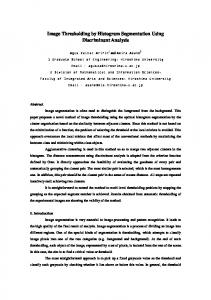
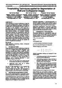
The segmented Fruits images obtained by the GbSA outperform the ones obtained by the GTASOM as reported in Table 7. Fig. 11 shows the segmented Fruits images obtained by the GbSA and the GTASOM. The high performance of the GbSA is clearly obvious in the figure. In contrast, Fig. 12 shows two segmented images produced by the GTASOM, which have better qualities than their counterparts produced by the GbSA. The shirt of the person behind the Hunter in Fig. 12(b) shows better uniformity than the one in Fig. 12(a). This fact is confirmed by the Edge-border Coincidence measures of the two segmented images reported in Table 7. Moreover, for the Couple image, the segmented image of Fig. 12(d) produced by the GTASOM shows higher quality than the one produced by the GbSA shown in Fig. 12(c). For example, the gray-levels above the door‘s frame and on the wall above the painting reflect better performance of the GTASOM in this figure. However, as it was mentioned earlier, the GbSA is generally more successful than the GTASOM for image segmentation.

(a)

(b)

(c)

(d)

(e)

(f)

To visually evaluate the performance of the proposed GbSA for multilevel thresholding, the segmented (thresholded) Lena images from one to eight thresholds are shown in Fig. 9. As the number of the thresholds increases, the segmented images become more similar to the original Lena image. Moreover, for the Peppers image, the thresholded images obtained by the GbSA and the iterative selection method are shown in Fig. 10. This figure shows the results for thresholding with five and eight thresholds. It is visually obvious that the images thresholded by the GbSA are better than those obtained by the iterative selection. The Otsu‘s values reported in Tables 1 and 2 also confirm the subjective judgment. Copyright © 2013 MECS

Fig. 11: The segmented (thresholded) Fruits images with the proposed GbSA and the GTASOM. (a)-(c) From left to right: Segmented images with the GbSA having four, eight, and 13 regions, respectively. (d)-(f) From left to right: Segmented images with the GTASOM having four, eight, and 13 regions, respectively


32


[2] P.Y. Yin. Multilevel minimum cross entropy threshold selection based on particle swarm optimization. Appl. Math. Comput, vol. 184, no. 2, 2007, pp. 503–513. [3] N.R. Pal, and S.K. Pal. A review on image segmentation techniques. Pattern Recognition, vol. 26, no. 9, 1993, pp. 1277–1294.

(a)

(b)

[4] N. Otsu. A threshold selection method from graylevel histogram. IEEE Trans. Systems Man Cybern., vol. 9, no. 1, 1979, pp. 62–66. [5] P.S. Liao, T.S. Chen, and P.C. Chung. A fast algorithm for multi-level thresholding. J. Inf. Sci. Eng., vol. 17, no. 5, 2001, pp. 713–727. [6] B. Biianu, S. Lee, and S. Das. Adaptive Image Segmentation Using Genetic and Hybrid Search Methods. IEEE Transactions on Aerospace and Electronic Systems, vol. 31, no. 4, 1995, pp. 12681291.

(c)

(d)

Fig. 12: The segmented (thresholded) images with the proposed GbSA and the GTASOM. (a) Segmented image with the GbSA having 16 regions. (b) Segmented image with the GTASOM having 16 regions. (c) Segmented image with the GbSA having 16 regions. (d) Segmented image with the GTASOM having 16 regions.

VII. Conclusions In this paper, a new metaheuristic for continuous optimization called ―Galaxy-based Search Algorithm‖ or GbSA is introduced. The proposed GbSA mimics the arms of spiral galaxies to search for the optimal solutions. It also uses a local search algorithm for fine tuning the solutions. Moreover, chaos plays an important role throughout the process of the GbSA. The GbSA is employed for optimizing the Otsu‘s criterion for multilevel thresholding of gray-level images. The performance of the GbSA for multilevel thresholding is compared with an exhaustive search and two other multilevel thresholding methods. The experiments reveal the superiority and fastness of the proposed GbSA. Due to the high performance of the GbSA for continuous optimization for multilevel thresholding, it is reasonable to employ the GbSA for other problems of Computer Vision and Image Processing in which objective functions are defined for optimization. It is noted that the GbSA has also been used for principal components analysis [28].

References [1] E. Zahara, S.K.S. Fan, and D.M. Tsai. Optimal multi-thresholding using a hybrid optimization approach. Pattern Recognition Letters, vol. 26, no. 8, 2005, pp. 1082–1095. Copyright © 2013 MECS

[7] L. Cao, P. Bao, and Z.K. Shi. The strongest schema learning GA and its application to multilevel thresholding. Image Vision and Computing, vol. 26, no. 5, 2008, pp. 716–724. [8] M. Maitra, and A. Chatterjee. A hybrid cooperative–comprehensive learning based PSO algorithm for image segmentation using multilevel thresholding. Expert Systems with Applications, vol. 34, no. 2, 2008, pp. 1341–1350. [9] H. Gao, W. Xu, J. Sun, and Y. Tang. Multilevel thresholding for image segmentation through an improved quantum-behaved particle swarm algorithm. IEEE Transactions On Instrumentation And Measurement, vol. 59, no. 4, 2010, pp. 934946. [10] W.B. Tao, H. Jin, and L.M. Liu. Object segmentation using ant colony optimization algorithm and fuzzy entropy. Pattern Recognition Letters, vol. 28, no. 7, 2008, pp. 788–796. [11] H. Shah-Hosseini. Intelligent Water Drops algorithm for automatic multilevel thresholding of gray-level images using a modified Otsu‘s criterion. International Journal of Modelling, Identification and Control, vol. 15, no. 4, 2012, pp. 241–249. [12] K. Hammouchea, M. Diaf, and P. Siarry. A comparative study of various meta-heuristic techniques applied to the multilevel thresholding problem. Engineering Applications of Artificial Intelligence, vol. 23, 2010, pp. 676–688. [13] H. Shah-Hosseini. Otsu‘s Criterion-based Multilevel Thresholding by a Nature-inspired Metaheuristic called Galaxy-based Search Algorithm. Third World Congress on Nature and Biologically Inspired Computing (NaBIC‘11), October 2011, Salamanca, Spain.



[14] E.H.L. Aarts and J.K. Lenstra. Local search in combinatorial optimization. In: Discrete Mathematics and Optimization, (Eds.), Wiley, Chichester, UK, 1997. [15] M. Sezgin and B. Sankur. Survey over image thresholding techniques and quantitative performance evaluation. Journal of Electronic Imaging, vol 13, no 1, 2004, pp. 146–165. [16] T.W. Ridler and S. Calvard. Picture thresholding using an iterative selection method. IEEE Trans. Systems, Man, and Cybernetics, vol. 8, no. 8, 1978, pp. 630-632. [17] H. Shah-Hosseini and R. Safabakhsh. TASOM: a new time adaptive self-organizing map. IEEE Transactions on Systems, Man and Cybernetics— Part B, vol. 33, no. 2, 2003, pp. 271–28. [18] H. Shah-Hosseini and R. Safabakhsh. Automatic multilevel thresholding for image segmentation by the growing time adaptive self-organizing map. IEEE Transactions on Pattern Analysis and Machine Intelligence, vol. 24, no. 10, 2002, pp. 1388–1393. [19] Y.J. Zhang. A survey on evaluation methods for image segmentation. Pattern Recognition, vol. 29, no. 8, 1996, pp. 1335-1346. [20] J.F. Canny. A computational approach to edge detection. IEEE Trans. Pattern Analysis and Machine Intelligence, vol. 8, no. 6, 1986, pp. 667698. [21] D.Y. Huang and C.H. Wang. Optimal multi-level thresholding using a two-stage Otsu optimization approach. Pattern Recognition Letters, vol. 30, no. 3, 2009, pp. 275–284.

33

[28] H. Shah-Hosseini. Principal components analysis by the galaxy-based search algorithm: a novel metaheuristic for continuous optimization. International Journal of Computational Science and Engineering, vol. 6, no.1/2, 2011, pp. 132 – 140.

Author’s Profile Hamed Shah-Hosseini was born in Tehran, Iran, in 1970. He received the B.S. degree in Computer Engineering from the University of Tehran. He also obtained the M.S. and Ph.D. degrees both in Computer Science (Artificial Intelligence) from the Amirkabir University of Technology, all with high honors. For seven years, he was an assistant professor in the Faculty of Electrical and Computer Engineering of Shahid Beheshti University. However, he could not continue his career there due to several non-academic conducts imposed on him. As a result, he is currently a freelance researcher. His research interests include Computational Intelligence especially Neural Networks, Evolutionary Computation, Swarm Intelligence, and Computer Vision. He proposed the Time-Adaptive SelfOrganizing Map (TASOM) networks for both stationary and nonstationary environments. Moreover, he introduced two nature-inspired optimization algorithms: ―Intelligent Water Drops‖ algorithm (or IWD algorithm) and ―Galaxy-based Search Algorithm‖ (or the GbSA). In addition, he presented a Generalized Taylor‘s (GTaylor‘s) Theorem.

[22] N. Mladenovic, and P. Hansen. Variable neighborhood search. Computers Operational Research, 1997, vol. 24, 1097-1100. [23] H.R. Lourenço, O. Martin and T. Stützle. Iterated Local Search. Handbook of Metaheuristics. Kluwer Academic Publishers, International Series in Operations Research & Management Science, vol. 57, 2003, pp. 321–353. [24] N. Krasnogor and J. Smith. A tutorial for competent memetic algorithms: model, taxonomy, and design issues. IEEE Transactions on Evolutionary Computation, vol. 9, no. 5, 2005, pp. 474–488. [25] J. Holland. Adaptation in natural and artificial systems. Ann Arbor: University of Michigan Press, 1975. [26] E. Ott, Chaos in Dynamical Systems, Cambridge, 2002. [27] USC-SIPI Image Database, 2012. Available at: http://sipi.usc.edu/database. Copyright © 2013 MECS
