Multilevel Thresholding Segmentation of T2 weighted Brain ... - arXiv

Multilevel Thresholding Segmentation of T2 weighted Brain MRI images using Convergent Heterogeneous Particle Swarm Optimization Mohammad Hamed Mozaffari1, Won-Sook Lee School of Electrical Engineering and Computer Science, University of Ottawa, 800 King-Edward Avenue, Ottawa, Ontario, Canada, K1N 7S6. Tel: +1-613-562-5800 ext. 2191

Abstract This paper proposes a new image thresholding segmentation approach using the heuristic method, Convergent Heterogeneous Particle Swarm Optimization algorithm. The proposed algorithm incorporates a new strategy of searching the problem space by dividing the swarm into subswarms. Each subswarm particles search for better solution separately lead to better exploitation while they cooperate with each other to find the best global position. The consequence of the aforementioned cooperation is better exploration, convergence and it able the algorithm to jump from local optimal solution to the better spots. A practical application of this method is demonstrated for the problem of medical image thresholding segmentation. We considered two classical thresholding techniques of Otsu and Kapur separately as the objective function for the optimization method and applied on a set of brain MR images. Comparative experimental results reveal that the proposed method outperforms another state of the art method from the literature in terms of accuracy, computation time and stable results. Keywords: Convergent Heterogeneous Particle Swarm Optimization; Multilevel Image Thresholding Segmentation; Otsu’s and Kapur’s criteria; Magnetic Resonance image; Multiswarm search.

1 Introduction Image processing techniques are used in any fields of science and technology such as astronomy, industry, and electronics. For medicine1–6, image processing is a vital tool that helps the physicians to interpret images of the patients to diagnose diseases easier and assist the surgeons to perform the operation with more accuracy and effectiveness. Generally, the goal of these techniques is to extract the valuable information in the images that is usually a critical and challenging task. Image segmentation is an absolutely essential preparatory process in almost all image processing approaches in which the image is divided into classes, the background, foreground and region of interest (ROI)7–9. As an optimum segmentation, pixels that contribute in each class should be similar in terms of gray- or RGB- level intensities. Thresholding methods10,11 are the easiest image segmentation approaches that in their simplest case (bi-level) endeavor to identify one optimum threshold value tb for the pixels intensity. Thus, the pixels whose intensity values are bigger than tb are labeled as the first class and the rest labeled as the second class, usually one class is for the background and another for the foreground region 1

Corresponding author Email address: [email protected] , [email protected]

1

of the image12,13. Multilevel thresholding is the extended version of the bi-level in which the image pixels are separated into more than two classes corresponding to threshold values. According to a prevalent taxonomy, thresholding methods are divided into parametric and nonparametric methods. In the parametric approaches, the gray-level distribution of each class leads to find the thresholds. In order to identify the model of each class, the parameters of the probability density function must be estimated. In the non-parametric techniques, optimizing one criteria such as the entropy, the error rate, and between-class variance results optimal threshold values12–16. Time-consuming and computationally expensive of the parametric methods cause that the non-parametric techniques become a desired and common alternative for the thresholding. For better results, criteria in these methods can also be considered as a fitness function for one optimization algorithm which is the main part of this study17. Amongst thresholding methods, Otsu’s 18–22 and Kapur’s 17,23,24 approach are two popular one because of their powerfulness, accuracy, and efficiency especially in the case of bi-level thresholding problem25. Although these classical methods perform well in bi-level thresholding problem but for multilevel thresholding problem, because of their exhaustive searching strategy, and greater dimension of the problem space, the computation time grows exponentially with increasing the number of thresholds26. Thus, in real-time multilevel thresholding applications, the classical methods are weak and necessity of new techniques is clear. Many studies try to find an alternative way to solve this issue and a common way is to consider multi-level thresholding as an optimization problem. Heuristic and Meta-heuristic optimization algorithms are known and distinguished for their fast and efficient performance. A combination of heuristic methods and classical thresholding methods not only can solve the problem of computation time, it also can increase the efficiency, accuracy, and robustness of the results27. Numerous heuristic techniques successfully have been used for the problem of multilevel thresholding segmentation. Heuristic optimization algorithms are inspired by the laws of physics, mechanics and mimic the developmental process in natural and biological phenomena such as Darwinian evolution in creations (Genetic Algorithm)15,28–30, crystal and molecular structure shaping in metallurgy (Simulated Annealing)31, foraging of ants (Ant Colony Optimization)32, social behaviours of flock of birds or school of fishes in migration (Particle Swarm Optimization)7,24,33– 45 , accumulation of water in catchment basins (Inclined Planes system Optimization)46,47 and numerous more examples. In order to use aforementioned techniques for thresholding segmentation problem, the common technique is to use the extended version of one classical thresholding method and consider it as a fitness (objective or criteria) function, then heuristic optimization method can find the best threshold values set iteratively by maximizing or minimizing that fitness function 8,28,48–50. In spite of the fact that heuristic methods are powerful enough in solving high dimensional problems but developing of these methods (better convergence, less sensitive to the parameters, more robust, more accurate and etc.) is still a hot topic for researchers. In this paper, application of a modified version of the Particle Swarm Optimization (PSO) algorithm with a new strategy of searching, named Convergence Heterogeneous Particle Swarm Optimization (CHPSO)51 on the problem of multi-level thresholding segmentation of Brain T-2 Magnetic Resonance (MR) images is investigated. Otsu’s and Kapur’s method is considered as the objective functions and 10 test images are used for the experiments. The experimental results reveal that the proposed method can reach to the best solution within fewer iteration numbers in comparison to the similar approaches without sticking into local solutions. The rest of the paper is organized as follows: In Section 2, the CHPSO algorithms are introduced with details. In Section 3, the Otsu's and Kapur's methods explained in details and Section 4 shows 2

experimental results and discussion about similar methods as a comparison study. Section 5 concludes the paper.

2 Methodology Heuristic optimization algorithms are designed for solving sophisticated optimization problems (non-linear in most cases) without having knowledge about the problem. Using a reasonable number of constant parameters, computation time and cost lead to an accurate and convergent optimal solution. In almost all heuristic optimization algorithms, there is a trade-off between two methodologies of exploration and exploitation which help the algorithm to search for the best solution efficiently and liberate from capturing in local optima as much as possible. Exploration reinforces algorithm to search the whole range of the problem space by expanding agents (particles) as far as possible in the search space while the exploitation enables the algorithm to find more accurate solutions with better searching locally. One of the most popular heuristic population-based optimization method is the Particle Swarm Optimization (PSO) which is inspired by the behavior of a flock of birds or a school of fishes during the migration and foraging which their social network helps them to find the best place of food and accommodation. The first version of this algorithm was very powerful and easy to implement, but since 1995 that the PSO algorithm was introduced33, many improvements have been suggested to update and enhance this method. Convergence Heterogeneous Particle Swarm Optimization (CHPSO) Algorithm41 is an enhanced version of the PSO which guarantees better optimal solution due to its new strategy of searching and better exploration and exploitation. In the following sections, the original version of the PSO and modified one CHPSO is explained clearly.

2.1 Particle Swarm Optimization In the PSO algorithm, cooperation between particles causes to find the best solution for the search space and each of them can be a candidate for that position. Particles are random selected in the initialization step, then each particle compares its current position with two relative information to update its position and move to a new position, iteratively. The criterion for comparison is the fitness function and the information is the personal best position from the previous iterations and the best position between particles acquired so far. The position and velocity of particles are calculated respect to this two information in each iteration. Thus, if the position and velocity of i  th particle in the time t and D dimensions are represented by X i  [ xi1 , xi2 ,, xiD ] , and Vi  [vi1 , vi2 ,, viD ] , respectively, then the position of the particle in the next iteration ( t  1 ) is updated according to the following equations. X i (t  1)  X i (t )  Vi (t  1) Vi (t  1)  Vi (t )  c1R( Pbesti (t )  X i (t ))  c2 R(Gbest(t )  X i (t ))

(1) (2)

where c1 and c2 are two constants for controlling the exploration and exploitation affects, respectively, R is uniformly distributed random vector from zero to one,  is an inertia weight constant which scales the effect of the velocity in the previous iteration, Pbesti (t ) and Gbest(t ) are the best personal position and the best position which have been acquired so far (from the time zero to t ). Note that the equations (1) and (2) are for the global version of the PSO and there is also the local version which is outside the scope of this report. 3

In a nutshell, for each particle, the corresponding score using the fitness function is calculated then the best personal particle position respect to the previous iteration is stored for using in the next iteration and also the best global particle position respect to the neighbor’s particles is selected. This is one of the advantages of the PSO that it needs just one stack of memory and there is no need to calculate complicated formula such as gradient which caused the PSO become a fast and easy to implement the algorithm. The pseudocode of the PSO is tabulated in Algorithm 1. Algorithm 1 The PSO algorithm pseudocode 1. Initialization. a. Set the constant parameters b. Randomize the vector of positions X and the velocities V of the particles in the search space c. Set the best personal position to current positions Pbest  X d.

Set

Gbest  arg{min f ( X )}

2. Termination Check. a. If the termination criterion is satisfied stop. The Gbest will be the output solution. b. Else go to Step 3. 3. For i  1,, number of iteration Do a. Update the velocity and position according to Equation (2) and (1) and check to be in the range space b. Evaluate fitness function of each particle. c. Save the best personal and global fitness value and position if better than previous End for Update the Gbest  arg{min f ( Pbest )} 4. Goto step 2

2.2 Convergent Heterogeneous Particle Swarm Optimization The ideal optimization algorithm with a perfect convergence and accurate solution (not local solutions) in a reasonable computational time and cost is always desirable and attracts many researchers from all fields of science to have a contribution in this area, at least, make an update to enhance previous optimization methods for a particular application. Depends on the search strategy of the optimization algorithm, trapping in local optimum solutions is an inevitable event and less probability of local trapping better results. For the particles of a fast convergent algorithm such as the original PSO, due to its homogeneous searching behavior (diversity of particles is lost) and their weak exploration ability, it is more likely for the algorithm to capture in local optimal spots within the first iterations. One way to solve this problem is to use a big coefficient for the exploration part of the algorithm at the expense of losing of exploitation effect and losing of accuracy. A new approach to solving this issue is to use multiswarm techniques which are designed to improve the exploration ability of the original heuristic optimization algorithms as well as the exploitation. Cheung et al.41 in 2014 proposed the CHPSO which uses the multiswarm technique to enhance the weakness of the PSO in jumping from local solutions to the global one. The main idea of the CHPSO is to divide particles into the four subswarms that each subswarm can search separately the problem space. Each subswarm moves heterogeneously in its local region but also share their information to the other two subswarms to explore new regions and specify the trajectory of the whole swarm in the solution domain. Totally, two subswarms are named basic subswarm which is used for exploitation search and the other two subswarms are called the adaptive subswarm and the exploration subswarm. The adaptive subswarm updates flight path adaptively with using the knowledge that was sent from the two basic subswarms in advanced. Unknown regions in the problem space are discovered by the exploration subswarm which uses 4

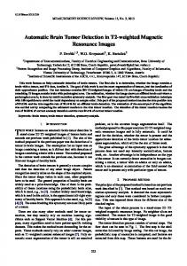
the information of the other three subswarms. Because, in CHPSO cooperation between particles is different from the original PSO, new update rules based on positions, velocities and the value of fitness function are defined for CHPSO and are added to the original PSO. As mentioned before, although each subswarm searches the problem space individually and shares its information with other subswarms (except exploration subswarm), it also contributes in the global exploitation which is the goal of the optimization algorithm. Consequently, all four subswarms search the problem space for the optimum solution heterogeneously while two of them (basic subswarms) supply their velocity and fitness values information for the adaptive subswarm for determining a better trajectory for all particles and finally the velocity information of these three subswarms are shared with the exploration subswarm to enable the algorithm to jump from local optima in order to find the areas of the problem space which never checked. For better understanding the particles situations, Figure 1 represents a schematic of four subswarms contain five particles that try to find the global best position of the two-dimensional function ( f ( x1 , x2 )  x12  x22 ). This cooperation between the particles is used for updating their positions in the next generation. As illustrated in Figure 1, for minimization problem like this, the global position Gbest is calculated according to the global position in the four subswarms and defined as equation (3).

Figure 1: A schematic of the CHPSO particles and their sharing information model applied on a 2D test function





Gbest  arg min f ( Pbest( sub( s )) | s  1,2,3,4)

(3)

where, Pbest ( sub( s )) is the best particle in subswarms. For updating the position of particles in the adaptive subswarm ( sub(3) ), the velocity and fitness function of the basic subswarms are needed and for updating the exploration subswarm ( sub(4) ) velocity of particles in the basic and adaptive subswarms are needed. Position updating rules for basic subswarms ( sub(1) and sub(2) ) and adaptive subswarm ( sub(1) ) are identical to the original PSO i.e. equations (1). The velocity of the basic subswarms is updated using equation (4). 5

Vi ( sub(1& 2)) (t  1)  Vi ( sub(1& 2)) (t )  c1R( Pi ( sub(1& 2)) (t )  X i ( sub(1& 2)) (t ))  c2 R(Gbest  X i ( sub(1& 2)) (t ))

(4)

where c1 and c2 are two constants for controlling the exploration and exploitation effects, respectively, R is uniformly distributed random vector from zero to one,  is an inertia weight constant which scales the effect of the velocity in the previous iteration, Pi ( sub(1&2)) (t ) and Gbest are the best personal position in the subswarm and the best position which have been gained so far (from the time zero to t ). Using the information are acquired from basic subswarms sub(1) and sub(2) , particles of the adaptive subswarm sub(3) can adjust the direction of the whole flight. Velocity of the i  th particle in the adaptive subswarm is updated using the following equation:     Vi ( sub( 3)) (t  1)    Vi ( sub(1)) (t  1)  Vi ( sub( 2 )) (t  1)  Vi ( sub( 3)) (t )   2   1   c1R( Pi ( sub( 3))  X i ( sub( 3)) (t ))  c2 R(Gbest  X i ( sub( 3)) (t ))    1   2

(5)

where  1 and  2 are the fitness values of the particles in the basic subswarms sub(1) and sub(2) , respectively and other parameters are similar to equation (2). The strategy of using  1 and  2 can be explained in this way that the subswarm with better fitness values has a larger effect on the particles in the adaptive subswarm. As discussed, particles of the subswarm sub(4) should attempt to explore new areas as far as possible from other subswarms, thus, the velocity of the i  th particle in the subswarm sub(4) is defined by the difference between the basic subswarms and adaptive one as the equation (6). The i  th particle position in subswarm sub(4) is updated according to its previous information and velocity of the i  th particle in the other subswarm as bellow: Vi ( sub( 4)) (t  1)  Vi ( sub(1)) (t  1)  Vi ( sub( 2)) (t  1)  Vi ( sub( 3)) (t  1) X i ( sub( 4)) (t  1)  1 X i ( sub( 4)) (t )   2 Pi ( sub( 4))  3Gbest  Vi ( sub( 4)) (t  1)

(6) (7)

where 1 ,  2 and 3 are named impact factors which indicate how much the previous information of the particle can contribute in updating process and they must satisfy this equation: 1  2  3  1 . The bigger impact factor 1 causes the previous information about the i  th particle effect more on updating process than information shared from other subswarms. Generally, diversity and fitness value of the particles in exploration subswarm is considerable because the particles use all the information in the whole swarm. In this paper, the impact factors 1 ,  2 and 3 are set to 1 6 , 1 and 1 , respectively. For better Understanding of the CHPSO algorithm, its pseudocode is 3 2

illustrated in Algorithm 1. Algorithm 2. The CHPSO algorithm pseudocode

1. Initialization. a. Set the constant parameters b. For i  1,...,4 do  Randomize the positions of all particles in subswarm i in the search space  Randomize the velocities of all particles in subswarm i in the search space

6

 c.

Set the Gbestsub(i )  arg{min f ( xisub(i ) )}

End For Set the swarm global Gbest  arg{min Gbestsub(1,2,3,4) }

2. Termination Check. a. If the termination criterion is satisfied stop. The Gbest will be the output solution. b. Else go to Step 3. 3. For i  1,, number of iteration Do For j  1,, number of particles Do a. Update the velocity and position of subswarms 1 and 2 according to Equation (4) and (1) and check to be in the range space b. Calculate  1 and  2 c. Update the velocity and position of subswarms 3 according to Equation (5) and (1) and check to be in the range space d. Update the velocity and position of subswarms 4 according to Equation (6) and (7) and check to be in the range space e. Evaluate fitness function of each subswarm and particles. f. Save the best subswarm personal and global fitness value and position if better than previous End for Update the Gbest  arg{min Gbestsub(1,2,3,4) } End for 4. Goto step 2

In the next chapter, using of the CHPSO for optimizing the Otsu and Kapur criteria is explained.

3 Otsu and Kapur Criteria The aim of image thresholding techniques is to find the optimal threshold values and can be defined and formulated as equations (8) and (9). Bi-level:

Multi-level:

 p(i , j )  S1 if   p(i , j )  S 2 if  p(i , j )  S1 if  p  (i , j )  S 2 if  p(i , j )  S k if    p(i , j )  S m if

0  p(i , j )  tb t b  p( i , j )  L  1

s

(8)

0  p(i , j )  t1 t1  p( i , j )  t2 t k  p( i , j )  t k  1

(9)

 t m  p( i , j )  L  1

where p(i , j ) , i  {1,2,..., r}, j  {1,2,..., c} is the pixel intensity of the image (with size r  c and with n  L gray levels from zero to L  1 ), t k is one of the selected different thresholds (in bi-level case k  b with just one threshold value and in the case of multi-level k  {1,2,  , L  1} with m number of desired thresholds), Sk is one of the sets in which pixels with intensities between thresholds t k and t k 1 are located. Otsu52 proposed a thresholding technique based on probability principles such as zero-, first- and second-order statistics to find the thresholds which can maximize between-class variance. To calculate the probability of each gray-level occurrence in the image, the number of the pixels with 7

that intensities is needed. Histogram diagram is a way to find this numbers as a gray-level distribution. The probability of each gray-level is determined by equation (10). hi  ,  Pri  Np  0  i  L  1, 

(10)

where hi is the value of histogram (the number of pixels with the specific intensity level i ), N p is the number of pixels in the image ( r  c ). In fact, equation (10) is the normalized version of the Np

histogram by N p and so 0  Pri  1,

 Pr  1 . i

i 1

Similar to the Otsu’s method, Kapur23 attempts to find the maximum entropy of the image after segmentation. Normalized Image histogram data again is used as the probability distribution of the pixels intensities. Equations for bi-level and multi-level Otsu’s and Kapur’s method are tabulated in Table 1 and Table 2, respectively. From the tables, the objective function that is used for the CHPSO is defined by equations (11) and (12) for Otsu’s and Kapur’s methods respectively. fitness(T )  max( 2 (T )), fitness(T )  max( H (T )),

(11) (12) where vector T  {t1, t2 , , tm }, 0  ti  L  1, i  1,2, , m (for bi-level value tb ) is a series of thresholds values. Table 1: Otsu’s method equations

Bi-level Image after thresholding Image is divided into two sets S1 and S2 (background and foreground pixels) using a threshold at the level tb , (m  1)

Multilevel Image after thresholding Image after thresholding is divided into m sets {S1 , S 2 , , S m } using thresholds at the levels

Classes Gray-levels

{t1, t2 , , tm } Classes Gray-levels S1  [0, ...,t1  1]

S1  [0, ...,tb  1]

S 2  [t1 , ...,t 2  1]

S 2  [tb , ..., L  1]

 S m  [t m , , L  1]

Probabilities distributions for each class

(k ) 

k 1

 Pr

i

(13)

i 0

8

t1  1

0 

0  1 

i

1 

b

i 0 L 1

i

  (t1 )

 Pr

i

  (t2 )   (t1 )

i 0 t 2 1

t b 1

 Pr  (t )

 Pr

i  t1

i



(14)

 Pr  ( L)  (t ) b

(15) L 1

 Pr

m 

i tb

1  2  1

  ( L )   (tm )

i

i tm m



i

1

i 0

Mean levels for each class

 (k ) 

k 1

i Pr

(16)

i

i 0

t1 1





 (t1 ) 0





 (t2 )   (t1 ) 1

0 

0  1 

tb 1



i 0 L 1

i Pri



0

i Pri

i  tb

1

 (tb )  0 

(17)

 ( L)   (tb ) 1

1 

i 0 t 2 1

i Pri 0

i Pri

i  t1

1

(18)



m 

L 1



i Pri

i tm



m

 ( L)   (tm ) m

Mean levels for the whole image

T 

L 1



i Pri   ( L) 

i 0

m

 

(19)

i i

i 0

The Otsu variance between classes  2   0 2   12  0 ( 0  T ) 2  1 ( 1  T ) 2

(20)

2 

m

m

   (   i

i 0

i

i

T)

2

(21)

i 0

Table 2: Kapur’s method equations

Bi-level Image after thresholding Image is divided into two sets S1 and S2 (background and foreground pixels) using a threshold at the level tb , (m  1) Classes Gray-levels

S1  [0, ...,tb  1] S 2  [tb , ..., L  1]

Multilevel Image after thresholding Image after thresholding Image is divided into m sets {S1 , S 2 , , S m } using thresholds at the levels {t1, t2 , , tm } Classes Gray-levels S1  [0, ...,t1  1]

S 2  [t1 , ...,t 2  1]  S m  [t m , , L  1]

The Kapur’s classes entropies

9

t1 1



ln(



ln(

H0 

H0 

t b 1



i 0 L 1

H1 

Pri 0



i  tb

ln(

Pri

ln(

1

Pri

0 Pri

1

)

(22) )

H1 

i 0 t 2 1

Pri 0

Pri

i  t1

1

Pri

)

Pri

)

0 1

(23)

 L 1

Hm 



Pri

i  tm

m

ln(

Pri

m

)

The Kapur’s overall entropy m

H  H1  H 2

(24)

H

H

(25)

i

i 0

In this paper, we proposed a combination of the CHPSO and these two criteria to find the best threshold values of the test image. In the next chapter, the application of the proposed method for medical image threshold segmentation is investigated and compared to the similar method.

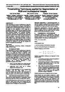
4 Experimental results and Discussion In order to evaluate the performance of the CHPSO, it has been applied on 10 benchmark images and the results compared with a novel heuristic algorithm named Amended Bacterial Foraging (ABF) algorithm53. Images are T2-weighted Brain-hemispheric MR and downloaded from the whole brain atlas database54. Transaxial slices from 22 to 112 with 10 slice gap interval are selected from the database. All the images have the same size ( 256  256 pixels) and they are in PNG format. A representation of the test images is depicted in Figure 2.

(a)

(b)

(c)

10

(d)

(e)

(f)

(g)

(h)

(i)

(j) Figure 2. Test images: A to J are Slices 22, 32, 43, 52, 63, 72, 82, 92, 102, 112, respectively. Since random numbers are used in the CHPSO algorithm like other heuristic methods in each run of the algorithm the outcome most likely to different from another run. Thus, it is valuable to employ an appropriate statistical metrics to measure the efficiency of the method. The results have been reported after executing the algorithm for 50 times for each image. It is common in the literature that the number of threshold points is selected from numbers 2, 3, 4, and 5. The number of iterations is set as stopping criteria for the CHPSO and there are not any limit for the best fitness values remains with no change. Therefore, algorithm run for the whole of the time interval and the parameters of the method are tabulated in

Table 3. We try to make a similar situation to the ABF method for better comparison.

Table 3. Parameters settings for CHPSOMT

11

Number of iteration 100

Number of particles 20

Acceleration constants 1.49 for both c1 and c2

Inertia weight Linearly is changed from 0.4 to 0.9

Calculating the Standard Deviation (STD) from equation (26) is a desirable way to show the dispersion of the data after 50 times repetition and minimum STD for algorithms the better stability.  N Bestfiti  Meanfit   STD     N  i 1 



(26)

where N is the number of algorithm run ( N  50) , bestfiti is the best fitness acquired from the i  th algorithm execution and Meanfit is the average result of all best finesses. Peak Signal to Noise Ratio (PSNR) is another way of assessing the proposed method in respect to quality and noise effects on the image. It compares the threshold delineated image with original one as a reference to find how much of original data are conveyed to the segmented image. The bigger PSNR the better signal quality and for defining the PSNR a common way is first to determine the mean squared error (MSE) by using both image data from the equation (27), then PSNR in decibels unit (dB) can be calculated by equation (28)17. MSE 

1 rc

r 1 c 1

 I (i, j)  I (i, j)

2

s

(27)

i 0 j 0

 255   PSNR  20 log10   MSE 

(28)

where r and c are the number of row and columns of gray-level original and segmented images ( I and I s ), respectively. In order to qualitatively assessment of the method, the results can be evaluated by the popular uniformity measure as equation (29)53. m

 ( f u 1 2m 

i

  j )2

j  0 i R j

N  ( f max  f min )

(29)

2

where, m is the number of thresholds, R j is the j  th region of the image that is segmented, f i is the gray level of the pixel i ,  j is the mean of the gray levels inside the region R j , N is the number of total pixels in the image, f min and f max are the minimum and maximum gray level of pixels within the image respectively. The value of the uniformity measure is between 0 and 1 29. Uniformity with higher value means the better thresholding. Also for having a comparison with ABF results, misclassification error (in present) which is the difference between the best thresholding with u  1 and the value calculated from equation (29) is considered as a criterion. The CHPSO is applied over the complete set of benchmark images first considering the Otsu’s method (equation (12) as the fitness function) and then using the Kapur’s method as the fitness function (equation (11)) to find the optimum thresholds. Note that, because of the CHPSO optimization algorithm has the type of minimization, fitness functions values are multiplied by minus to change the problem space from maximization to minimization. 12

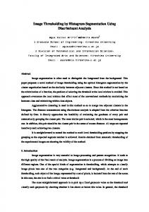
A visualization of the results after applying the proposed method on the images are illustrated in Figure 3 and Figure 4 using Otsu’s and Kapur’s criteria, respectively. As we can see in the figures, the white matter, gray matter, and cerebrospinal fluid are delineated perfectly with more details. In the case of the bigger number of thresholds, the quality of the image is significantly considerable and reveals that the proposed method can save similar patterns in the original image and convey them to the segmented one. In medical applications, the details in the images mean better diagnosis and better treatment and the images proof that our method can be used for this purposes.

Slice 022 (a)

(b)

(c)

(d)

Slice 032 (a)

(b)

(c)

(d)

Slice 042 (a)

(b)

(c)

(d)

Slice 052 (a)

(b)

(c)

(d)

13

Slice 062 (a)

(b)

(c)

(d)

Slice 072 (a)

(b)

(c)

(d)

Slice 082 (a)

(b)

(c)

(d)

Slice 092 (a)

(b)

(c)

(d)

Slice 102 (a)

(b)

(c)

(d)

14

Slice 112 (a)

(b)

(c)

(d)

Figure 3. CHPSO results using Otsu’s method – (a to d) are images after thresholding with m = 2, 3, 4 and 5, respectively

Slice 022 (a)

(b)

(c)

(d)

Slice 032 (a)

(b)

(c)

(d)

Slice 042 (a)

(b)

(c)

(d)

15

Slice 052 (a)

(b)

(c)

(d)

Slice 062 (a)

(b)

(c)

(d)

Slice 072 (a)

(b)

(c)

(d)

Slice 082 (a)

(b)

(c)

(d)

Slice 092 (a)

(b)

(c)

(d)

16

Slice 102 (a)

(b)

(c)

(d)

Slice 112 (a)

(b)

(c)

(d)

Figure 4. CHPSO results using Kapur’s method – (a to d) are images after thresholding with m = 2, 3, 4 and 5, respectively

The performance of the CHPSO for image thresholding was astonishing and clearly shows the powerfulness of this method, but this results should be compared with other similar techniques to figure out the advantages and disadvantages of the CHPSO. For this reason, the results of the ABF algorithm are tabulated beside the CHPSO in the following tables. From the Table 4, we can assert that two methods have a similar amount of fitness function, especially for Kapur’s method. In the case of Otsu, the results of the two proposed method are different but they could converge well. The difference between this results is that no pre- or postprocessing have been done on the images for the case of CHPSO. For instance, we can see threshold value of 0 in the slice 112 that is because in the original image there is a line with zero intensity. Table 4. Comparison study of threshold and fitness function values obtained by CHPSO and ABF using Otsu and Kapur

image

Slice22

Slice32

Slice42

Slice52

Slice62 Slice72

m 2 3 4 5 2 3 4 5 2 3 4 5 2 3 4 5 2 3 4 5 2

CHPSO Otsu Optimum Thresholds values 35,99 22,66,117 16,51,88,128 14,42,73,105,140 43,112 23,69,122 18,58,96,135 17,51,84,116,150 45,121 30,81,135 23,67,113,161 18,55,91,128,174 45,115 36,88,132 19,58,97,137 18,57,92,125,164 46,123 39,96,147 35,84,122,169 19,58,96,132,179 45,126

Fitness function 2273.7 2370.3 2409.3 2429.2 2607.1 2712.4 2751.8 2773.8 3044.4 3143.9 3199.7 3234.6 2858.8 2946.9 2997.4 3023.6 3369.4 3484.6 3537.5 3577.9 3206.2

Kapur Optimum Thresholds values 94,182 56,114,184 47,96,146,192 41,83,124,170,205 108,184 52,114,184 38,84,132,188 33,77,121,168,203 112,182 82,130,186 28,75,126,186 26,71,116,162,201 116,184 108,164,202 83,124,167,206 25,69,117,165,203 120,186 100,146,194 86,126,169,207 28,72,117,161,201 116,178

Fitness function 9.2155 11.733 13.946 16.105 9.2645 11.683 13.936 16.043 9.2585 11.578 13.865 16.026 9.2447 11.58 13.734 15.874 9.3367 11.674 13.77 15.866 9.4205

ABF Otsu Optimum Thresholds values 93,176 68,118,188 45,109,160,184 47,90,128,174,191 107,178 68,125,168 51,94,129,188 45,79,115,152,194 112,182 78,127,178 57,112,138,177 53,90,126,162,202 118,188 98,130,176 84,109,140,180 59,99,129,162,206 118,183 94,132,186 78,118,151,198 75,102,130,162,201 111,173

Fitness function 1808.8478 2165.1669 2288.3476 2321.4811 1809.3391 2557.1341 2672.3691 2714.2533 2118.4914 2891.0697 3120.0412 3166.4774 1569.4257 2099.4181 2488.3868 2934.7700 2158.5697 2781.2290 3217.2777 3312.1446 2082.9210

Kapur Optimum Thresholds values 95,184 68,115,186 43,89,136,186 44,85,127,173,207 110,185 82,130,190 44,92,136,188 42,92,134,184,216 114,184 83,136,187 48,102,144,190 40,93,137,183,217 117,186 109,163,203 92,131,173,210 48,89,131,175,209 119,186 99,150,195 93,134,176,212 82,114,147,181,216 117,179

Fitness function 9.2155 11.7123 13.9481 16.2228 9.2644 11.6166 13.9222 16.0040 9.2585 11.5743 13.8155 15.9644 9.2447 11.5552 13.7502 15.7152 9.3314 11.6688 13.7812 15.6953 9.4205

17

Slice82

Slice92

Slice102

Slice112

40,103,164 36,87,124,182 21,60,94,130,185 45,125 42,105,171 35,83,119,181 19,58,92,127,187 43,113 39,95,136 19,59,99,140 18,56,89,116,155 43,112 39,95,142 20,60,101,146 19,57,90,119,158 41,110 26,74,127 22,65,102,147 19,55,84,112,154

3 4 5 2 3 4 5 2 3 4 5 2 3 4 5 2 3 4 5

3342.1 3405.5 3441.5 2938.1 3061.3 3117.1 3151.6 2654 2716.1 2750.7 2775.5 2571.6 2643.6 2682.7 2703.9 2016.6 2090.2 2126.7 2141.1

98,140,186 95,134,174,213 47,88,129,169,208 110,168 102,144,188 84,122,161,203 33,79,123,164,202 108,172 104,156,204 85,126,165,206 29,78,120,165,206 106,172 92,140,188 31,85,135,182 16,71,111,151,193 104,162 1,70,141 0,65,122,170 0,49,95,138,182

11.694 13.846 15.797 9.191 11.427 13.508 15.564 8.7906 11.164 13.276 15.376 8.5283 10.928 13.067 15.31 8.1476 10.601 13.058 15.281

103,145,196 99,126,159,201 75,100,130,168,209 115,167 108,145,200 98,126,145,198 87,107,131,162,212 100,182 97,141,193 90,120,156,191 88,110,137,166,208 100,158 93,139,184 91,126,147,206 84,110,139,179,206 93,170 78,124,181 72,104,144,182 60,95,130,168,196

2270.0114 2452.8171 3137.3314 1653.4012 1826.7544 2111.0125 2505.4256 1612.4944 1671.3594 1971.2016 1993.7386 1732.1681 1851.2240 2000.5093 2127.9426 1843.8040 1907.0305 1973.3334 2039.0589

99,145,196 99,140,179,214 84,116,148,179,215 111,170 103,146,194 95,131,170,210 91,123,158,189,220 109,174 105,159,207 97,135,174,212 92,123,155,186,216 108,174 95,143,190 89,132,170,204 85,122,154,186,217 105,164 74,130,176 47,96,141,184 50,99,140,175,208

11.6758 13.9463 15.8427 9.1910 11.4140 13.6188 15.4033 8.7906 11.1560 13.2974 15.2733 8.5283 10.9375 13.0186 14.8850 8.1476 10.4500 12.7611 14.6592

Although, the results for the Otsu’s methods is different but we can compare them in terms of statistical analysis. In terms of the Standard deviation, the Peak Signal to Noise Ratio, we can understand from Table 5 that the CHPSO is highly robustness and in almost all cases gained a better STD rather than ABF and consequently more trustable respect to changes of output in each execution of the algorithm. The difference of PSNR for all images about 2 times bigger, reveal another property of the proposed method. The performance of the CHPSO in skipping from the local minima to better solutions lead to outstanding results in compare to the ABF and proof the power of multiswarm optimization algorithms for better exploration of the search space. Table 5. Comparison study of the CHPSO and ABF in terms of STD and PSNR

image

Slice22

Slice32

Slice42

Slice52

Slice62

Slice72

Slice82

m 2 3 4 5 2 3 4 5 2 3 4 5 2 3 4 5 2 3 4 5 2 3 4 5 2 3

CHPSO Otsu STD 0 2.2968e-12 1.3781e-12 3.1395 2.7562e-12 1.8375e-12 3.6749e-12 0.18787 1.3781e-12 0 0.016243 0.0082017 9.1873e-13 9.1873e-13 0.0042822 0.1792 4.5936e-12 2.2968e-12 3.6749e-12 0.66916 2.7562e-12 2.2968e-12 1.3781e-12 0.017521 2.7562e-12 4.5936e-13

PSNR 24.5006 24.6694 24.8633 25.6535 24.4469 24.5709 24.7943 24.9692 24.3693 24.5606 24.7001 24.8189 24.4490 24.6998 24.7770 24.9605 24.3949 24.6499 24.8458 24.8808 24.3542 24.5795 24.8080 24.8603 24.3593 24.5585

Kapur STD 1.0766e-14 5.3832e-15 0.011992 0.049308 7.1776e-15 1.0766e-14 0.023538 0.013657 8.972e-15 8.972e-15 0.00032519 0.0073274 5.3832e-15 8.972e-15 0.048056 0.046858 3.5888e-15 5.3832e-15 0.036804 0.080143 8.972e-15 8.972e-15 0.00020507 0.053892 5.3832e-15 3.5888e-15

PSNR 24.269 24.416 24.573 24.654 24.315 24.444 24.567 24.674 24.339 24.443 24.585 24.68 24.359 24.479 24.661 24.698 24.354 24.574 24.718 24.77 24.358 24.597 24.656 24.794 24.427 24.59

ABF Otsu STD 0.0021 0.7238 0.8222 1.0210 0.3119 0.4844 0.5001 0.5313 0.2813 0.4063 0.7813 1.2969 0.1278 0.5000 0.9375 1.7656 0.1474 1.0001 1.2031 1.8906 0.2594 0.5156 0.6875 1.0625 0.2731 1.1406

PSNR 10.0804 13.4236 15.5969 16.8073 9.1680 12.5778 15.5448 17.2658 9.0416 12.4376 15.0468 15.9160 9.1512 9.9752 11.4083 15.4337 9.1676 10.7943 11.1523 13.8409 8.9376 10.7279 11.1622 11.8284 9.4512 10.0912

Kapur STD 1.1721e-4 0.0009 0.0021 0.0165 1.0022e-4 0.0018 0.0111 0.0329 1.5000e-4 0.0175 0.0527 0.0729 1.3018e-4 0.0015 0.068 0.0996 1.1012e-4 0.0047 0.0169 0.0867 5.5610e-5 0.0097 0.0378 0.0642 2.7307e-4 0.0049

PSNR 10.3797 13.4504 16.2311 17.7098 9.2958 13.2597 16.9498 17.3335 9.0892 12.9165 16.3489 17.7189 9.2423 10.3772 11.9692 16.8916 9.2923 11.0396 11.9759 14.8511 9.4718 11.0624 11.7246 12.6370 9.7528 10.5192

18

Slice92

Slice102

Slice112

4 5 2 3 4 5 2 3 4 5 2 3 4 5

9.1873e-13 0.014472 3.6749e-12 1.8375e-12 1.3781e-12 0.017778 3.2155e-12 2.7562e-12 1.3781e-12 0.78066 1.1484e-12 1.3781e-12 1.3781e-12 0.020992

24.7953 24.8838 24.3605 24.7015 24.6962 24.9622 24.3440 24.5524 24.5521 24.7973 24.3324 24.3872 24.5038 24.6291

0.027152 0.11362 8.972e-15 0 0.05869 0.13649 8.972e-15 0 0.091335 0.21657 5.3832e-15 0.013084 0.0019779 0.0090181

24.741 24.716 24.365 24.46 24.699 24.68 24.327 24.512 24.672 24.914 24.296 29.42 29.672 30.25

1.5781 1.8594 0.5419 1.3438 2.0000 2.4375 0.2828 1.0056 1.1406 1.2656 0.2920 0.8281 1.5469 1.8156

11.0186 12.2378 9.2776 9.8622 10.5923 10.8404 9.3085 10.5222 11.1791 11.8127 9.0078 12.5501 12.8380 14.9048

0.0318 0.0508 1.6631e-4 0.0117 0.0248 0.0438 5.9248e-5 0.0031 0.0045 0.0099 0.0022 0.0057 0.0098 0.0367

11.2897 12.7024 9.7164 10.2338 10.9162 11.4210 9.3821 10.6334 11.2439 12.6854 9.0723 12.8712 15.9141 16.5306

From the Error! Not a valid bookmark self-reference., we can see that the CHPSO is also significantly faster than ABF algorithm. In this report, the algorithm is implemented using MATLAB software on the PC with a dual core of 3GHz with 2 GB memory. Faster results mean the ability of the proposed method for using in the real-time application that is common in medicine. In term of misclassification error in percentage, CHPSO could achieve better results in most cases especially when the number of thresholds is five. For the sake of representation the results of only three and five thresholds values are illustrated in

Table 7. In general, the experimental results reveals that the CHPSO approach using both Otsu and Kapur’s criteria is a robust, fast and accurate for the problem of medical image thresholding segmentation in comparison to the similar methods. The CHPSO for getting perfect results owe to the multiswarm searching strategy and the behavior of the particles that able them to search more new regions in the problem space and jump from local minima to a global one and discover a bigger area. For the speed of the algorithm, it was predictable, because of the simple equations of the original PSO that have not any complex calculations. Table 6. Comparison study of CHPSO and ABF in term of computation time (Ct) in second image

Slice22

Slice32

Slice42

Slice52

Slice62

Slice72

m 2 3 4 5 2 3 4 5 2 3 4 5 2 3 4 5 2 3 4 5 2 3

CHPSO Ct Otsu 0.1358 0.1353 0.1334 0.1313 0.1375 0.1347 0.1352 0.1313 0.1347 0.1347 0.1347 0.1333 0.1362 0.1352 0.1346 0.1313 0.1353 0.1351 0.1341 0.1301 0.1344 0.1361

Ct Kapur 0.28989 0.29003 0.27506 0.26038 0.28806 0.28466 0.27242 0.2554 0.28964 0.27923 0.27337 0.255 0.28743 0.28174 0.27972 0.25377 0.30375 0.27951 0.28061 0.25346 0.29204 0.27807

ABF Ct Otsu 3.0993 3.2681 3.7904 3.9115 2.7974 3.2821 3.9708 4.6637 2.7200 3.2588 3.8201 4.5712 2.7831 3.3111 3.6868 4.4951 2.9800 3.2259 3.2801 4.8114 2.7206 3.0875

Ct Kapur 6.5245 6.9201 7.4347 8.1779 6.7466 7.2019 7.5040 8.1982 6.7982 7.1599 7.8631 8.1029 6.7001 7.0938 7.2184 8.2670 6.5281 6.8914 7.1803 8.1060 6.6929 7.3030

19

4 5 2 3 4 5 2 3 4 5 2 3 4 5 2 3 4 5

Slice82

Slice92

Slice102

Slice112

0.1373 0.1324 0.1354 0.1347 0.1347 0.1322 0.1352 0.1340 0.1329 0.1311 0.1340 0.1344 0.1397 0.1336 0.1375 0.1372 0.1362 0.1349

0.26924 0.25184 0.28678 0.28047 0.26758 0.24793 0.28497 0.28531 0.26767 0.2597 0.28779 0.2829 0.25795 0.23269 0.28855 0.24958 0.24055 0.22548

3.8888 4.6753 2.8140 3.1250 3.6752 4.2175 2.7547 2.9126 3.8376 4.3922 2.6866 3.1403 3.5517 4.4888 2.8102 2.9396 4.1515 4.6141

7.4115 8.3934 6.6602 7.4265 7.5396 7.8576 6.4305 7.2827 7.6173 8.1403 6.6314 7.0547 7.2156 7.8035 6.5551 7.2357 7.5813 7.9576

Table 7. Comparison study of CHPSO and ABF in term of misclassification error in percentage (ME) Image Slice 022 Slice 032 Slice 042 Slice 052 Slice 062 Slice 072 Slice 082 Slice 092 Slice 102 Slice 112

m 3 5 3 5 3 5 3 5 3 5 3 5 3 5 3 5 3 5 3 5

CHPSO ME (in %) Otsu 0.1578 0.0744 0.1312 0.0900 0.2319 0.0999 0.3038 0.0772 0.3095 0.0675 0.2954 0.0735 0.3304 0.0542 0.2265 0.0476 0.2475 0.0465 0.0849 0.0479

ME (in %) Kapur 1.4977 1.2437 1.1307 0.5876 3.6760 0.2194 11.6213 0.1719 9.2941 0.2305 9.7454 0.7059 11.2282 0.2791 11.8704 0.1634 7.9017 0.0231 0 0

ABF ME (in %) Otsu 1.98 1.4 1.82 0.85 3.24 1.1 8.03 1.33 7.47 4.33 10.98 4.97 12.27 9.02 9.49 5.53 7.25 5.49 1.77 1.11

ME (in %) Kapur 2.04 1.14 2.18 1.01 3.05 1.27 9.16 1.40 7.73 5.57 8.01 4.31 12.33 7.24 10.29 5.97 7.63 6.98 2.38 1.59

5 Conclusion This paper has presented a new approach for thresholding segmentation of MR brain images using a combination of Convergent Heterogeneous Particle Swarm Optimization (CHPSO) and two classical thresholding techniques. We have shown that utilizing a new strategy of searching named multiswarm can improve the performance of a heuristic algorithm for the problem of image thresholding. In this strategy, the particles are divided into subswarms and each subswarm separately searches the problem space to find the best solution and improve the exploitation while the subswarms have a cooperation with each other and share their information for better exploration to find the global best position and jump from local optimal answers. Empirical testing on a set of 10 medical images, shows that the proposed approach is significantly robustness with better convergence, in comparison to similar techniques. Instead of reporting classical techniques, we compare our method with the state of the art and powerful heuristic 20

method Amended Bacterial Foraging (ABF). In terms of speed and accuracy also, the CHPSO outperforms the ABF. For visualization of the results, all segmented images have been illustrated. Images show that the details form the original image properly conveyed into the segmented image with more details. In future work, we hope to apply other kinds of multiswarm heuristic algorithms and provide more obvious demonstrations of this technique by applying it to more complex kinds of segmentation and images.

References 1.

2. 3.

4.

5.

6.

7. 8.

9.

10. 11. 12. 13.

14. 15.

Hamamci A, Kucuk N, Karaman K, Engin K, Unal G. Tumor-cut: segmentation of brain tumors on contrast enhanced MR images for radiosurgery applications. Med Imaging, IEEE Trans. 2012;31(3):790-804. Banerjee S, Mitra S, Shankar BU. Single seed delineation of brain tumor using multithresholding. Inf Sci (Ny). 2016;330:88-103. Balan NS, Kumar AS, Raja NSM, Rajinikanth V. Optimal Multilevel Image Thresholding to Improve the Visibility of Plasmodium sp. in Blood Smear Images. In: Proceedings of the International Conference on Soft Computing Systems. ; 2016:563-571. Dawngliana M, Deb D, Handique M, Roy S. Automatic brain tumor segmentation in MRI: Hybridized multilevel thresholding and level set. In: Advanced Computing and Communication (ISACC), 2015 International Symposium on. ; 2015:219-223. Remamany KP, Chelliah T, Chandrasekaran K, Subramanian K. Brain Tumor Segmentation in MRI Images Using Integrated Modified PSO-Fuzzy Approach. Int Arab J Inf Technol. 2015;12. Feng Y, Shen X, Chen H, Zhang X. Internal Generative Mechanism Based Otsu Multilevel Thresholding Segmentation for Medical Brain Images. In: Advances in Multimedia Information Processing--PCM 2015. Springer; 2015:3-12. Akay B. A study on particle swarm optimization and artificial bee colony algorithms for multilevel thresholding. Appl Soft Comput. 2013;13(6):3066-3091. Zhou C, Tian L, Zhao H, Zhao K. A method of two-dimensional Otsu image threshold segmentation based on improved firefly algorithm. In: Cyber Technology in Automation, Control, and Intelligent Systems (CYBER), 2015 IEEE International Conference on. ; 2015:1420-1424. Bhandari AK, Kumar A, Singh GK. Modified artificial bee colony based computationally efficient multilevel thresholding for satellite image segmentation using Kapur’s, Otsu and Tsallis functions. Expert Syst Appl. 2015;42(3):1573-1601. Sezgin M, others. Survey over image thresholding techniques and quantitative performance evaluation. J Electron Imaging. 2004;13(1):146-168. Liu Y, Xue J, Li H. The Study on the Image Thresholding Segmentation Algorithm. 2015. Horng M-H. Multilevel thresholding selection based on the artificial bee colony algorithm for image segmentation. Expert Syst Appl. 2011;38(11):13785-13791. Ayala HVH, dos Santos FM, Mariani VC, dos Santos Coelho L. Image thresholding segmentation based on a novel beta differential evolution approach. Expert Syst Appl. 2015;42(4):2136-2142. Oliva D, Cuevas E, Pajares G, Zaldivar D, Osuna V. A multilevel thresholding algorithm using electromagnetism optimization. Neurocomputing. 2014;139:357-381. Hammouche K, Diaf M, Siarry P. A multilevel automatic thresholding method based on a genetic algorithm for a fast image segmentation. Comput Vis Image Underst. 21

16. 17.

18. 19. 20. 21.

22. 23.

24.

25. 26.

27. 28. 29. 30. 31.

32. 33. 34.

2008;109(2):163-175. Horng MH. A multilevel image thresholding using the honey bee mating optimization. Appl Math Comput. 2010;215(9):3302-3310. doi:10.1016/j.amc.2009.10.018. Cuevas E, Zaldívar D, Perez-Cisneros M. Otsu and Kapur Segmentation Based on Harmony Search Optimization. In: Applications of Evolutionary Computation in Image Processing and Pattern Recognition. Springer; 2016:169-202. Otsu N. A threshold selection method from gray-level histograms. Automatica. 1975;11(285-296):23-27. Vala HJ, Baxi A. A review on Otsu image segmentation algorithm. Int J Adv Res Comput Eng Technol. 2013;2(2):pp - 387. Bindu CH, Prasad KS. An efficient medical image segmentation using conventional OTSU method. Int J Adv Sci Technol. 2012;38:67-74. Huang M, Yu W, Zhu D. An improved image segmentation algorithm based on the Otsu method. In: Software Engineering, Artificial Intelligence, Networking and Parallel & Distributed Computing (SNPD), 2012 13th ACIS International Conference on. ; 2012:135139. Huang D-Y, Wang C-H. Optimal multi-level thresholding using a two-stage Otsu optimization approach. Pattern Recognit Lett. 2009;30(3):275-284. Kapur JN, Sahoo PK, Wong AKC. A new method for gray-level picture thresholding using the entropy of the histogram. Comput Vision, Graph Image Process. 1985;29(1):140. doi:10.1016/0734-189X(85)90125-2. Banerjee S, Jana ND. Bi level kapurs entropy based image segmentation using particle swarm optimization. In: Computer, Communication, Control and Information Technology (C3IT), 2015 Third International Conference on. ; 2015:1-4. Oliva D, Cuevas E, Pajares G, Zaldivar D, Perez-Cisneros M. Multilevel thresholding segmentation based on harmony search optimization. J Appl Math. 2013;2013. Gao H, Xu W, Sun J, Tang Y. Multilevel thresholding for image segmentation through an improved quantum-behaved particle swarm algorithm. Instrum Meas IEEE Trans. 2010;59(4):934-946. Hammouche K, Diaf M, Siarry P. A comparative study of various meta-heuristic techniques applied to the multilevel thresholding problem. Eng Appl Artif Intell. 2010;23(5):676-688. Fu Z, He JF, Cui R, et al. Image Segmentation with Multilevel Threshold of Gray-Level & Gradient-Magnitude Entropy Based on Genetic Algorithm. psq. 2015;255:9. Yin P-Y. A fast scheme for optimal thresholding using genetic algorithms. Signal Processing. 1999;72(2):85-95. Sun G, Zhang A, Yao Y, Wang Z. A novel hybrid algorithm of gravitational search algorithm with genetic algorithm for multi-level thresholding. Appl Soft Comput. 2016. Zhang Y, Yan H, Zou X, Tao F, Zhang L. Image Threshold Processing Based on Simulated Annealing and OTSU Method. In: Proceedings of the 2015 Chinese Intelligent Systems Conference. ; 2016:223-231. Kaur U, Sharma R, Dosanjh M. Cancers Tumor Detection using Magnetic Resonance Imaging with Ant Colony Algorithm. Eberhart R, Kennedy J. A new optimizer using particle swarm theory. MHS’95 Proc Sixth Int Symp Micro Mach Hum Sci. 1995:39-43. doi:10.1109/MHS.1995.494215. Hamdaoui F, Ladgham A, Sakly A, Mtibaa A. A new images segmentation method based on modified particle swarm optimization algorithm. Int J Imaging Syst Technol. 2013;23(3):265-271. 22

35.

36.

37.

38. 39. 40.

41.

42.

43.

44.

45.

46.

47.

48.

49. 50.

Ait-Aoudia S, Guerrout E-H, Mahiou R. Medical Image Segmentation Using Particle Swarm Optimization. In: Information Visualisation (IV), 2014 18th International Conference on. ; 2014:287-291. Wei K, Zhang T, Shen X, Liu J. An improved threshold selection algorithm based on particle swarm optimization for image segmentation. In: Natural Computation, 2007. ICNC 2007. Third International Conference on. Vol 5. ; 2007:591-594. Mishra D, Bose I, De UC, Das M. Medical Image Thresholding Using Particle Swarm Optimization. In: Intelligent Computing, Communication and Devices. Springer; 2015:379383. Esmin AAA, Coelho RA, Matwin S. A review on particle swarm optimization algorithm and its variants to clustering high-dimensional data. Artif Intell Rev. 2015;44(1):23-45. Liu Y, Mu C, Kou W, Liu J. Modified particle swarm optimization-based multilevel thresholding for image segmentation. Soft Comput. 2015;19(5):1311-1327. Sayed GI, Hassanien AE. Abdominal CT Liver Parenchyma Segmentation Based on Particle Swarm Optimization. In: The 1st International Conference on Advanced Intelligent System and Informatics (AISI2015), November 28-30, 2015, Beni Suef, Egypt. ; 2016:219228. Cheung NJ, Ding X-M, Shen H-B. OptiFel: A convergent heterogeneous particle swarm optimization algorithm for Takagi--Sugeno fuzzy modeling. Fuzzy Syst IEEE Trans. 2014;22(4):919-933. Eberhart RC, Shi Y. Particle swarm optimization: developments, applications and resources. In: Evolutionary Computation, 2001. Proceedings of the 2001 Congress on. Vol 1. ; 2001:81-86. Song M-P, Gu G-C. Research on particle swarm optimization: a review. In: Machine Learning and Cybernetics, 2004. Proceedings of 2004 International Conference on. Vol 4. ; 2004:2236-2241. Li Y, Jiao L, Shang R, Stolkin R. Dynamic-context cooperative quantum-behaved particle swarm optimization based on multilevel thresholding applied to medical image segmentation. Inf Sci (Ny). 2015;294:408-422. Muthiah-Nakarajan V, Noel MM. Galactic Swarm Optimization: A new global optimization metaheuristic inspired by galactic motion. Appl Soft Comput J. 2016;38:771-787. doi:10.1016/j.asoc.2015.10.034. Mozaffari MH, Zahiri SH. UNSUPERVISED DATA AND HISTOGRAM CLUSTERING USING INCLINED PLANES SYSTEM OPTIMIZATION ALGORITHM. Image Anal Stereol. 2014;33(1). Mozaffari MH, Abdy H, Zahiri SH. Application of inclined planes system optimization on data clustering. In: Pattern Recognition and Image Analysis (PRIA), 2013 First Iranian Conference on. ; 2013:1-3. Pal SS, Kumar S, Kashyap M, Choudhary Y, Bhattacharya M. Multi-level Thresholding Segmentation Approach Based on Spider Monkey Optimization Algorithm. In: Proceedings of the Second International Conference on Computer and Communication Technologies. ; 2016:273-287. Sathya PD, Kayalvizhi R. Optimal multilevel thresholding using bacterial foraging algorithm. Expert Syst Appl. 2011;38(12):15549-15564. doi:10.1016/j.eswa.2011.06.004. Rajinikanth V, Raja NSM, Satapathy SC. Robust Color Image Multi-thresholding Using Between-Class Variance and Cuckoo Search Algorithm. In: Information Systems Design and Intelligent Applications. Springer; 2016:379-386. 23

51.

52. 53. 54.

Cheung A, Ding X-M, Shen H-B. OptiFel: A Convergent Heterogeneous Particle Swarm Optimization Algorithm for Takagi-Sugeno Fuzzy Modeling. IEEE Trans Fuzzy Syst. 2013;PP(99):1-1. doi:10.1109/TFUZZ.2013.2278972. Otsu N, Smith PL, Reid DB, et al. A Tlreshold Selection Method from Gray-Level Histograms. 1979;20(1):62-66. Sathya PD, Kayalvizhi R. Amended bacterial foraging algorithm for multilevel thresholding of magnetic resonance brain images. Measurement. 2011;44(10):1828-1848. Johnson KA, Becker JA, Williams L. The whole brain atlas. 1999.

24