multi objective design space exploration for grid alu processor

International Journal of Embedded Systems and Applications (IJESA) Vol.2, No.3, September 2012

MULTI OBJECTIVE DESIGN SPACE EXPLORATION FOR GRID ALU PROCESSOR Reza Asgari1, Ali Ahmadian Ramaki2, Reza Ebrahimi Atani3 and Asadollah Shahbahrami 4 1

Department of Computer Engineering, Guilan University, Rasht, Iran [email protected]

2

Department of Computer Engineering, Guilan University, Rasht, Iran [email protected]

3

Department of Computer Engineering, Guilan University, Rasht, Iran

4

Department of Computer Engineering, Guilan University, Rasht, Iran

[email protected] [email protected]

ABSTRACT Todays billions of transistors allow architects to design different huge processor to increasing parallel execution of instructions, which leads to increasing complexity of architecture. Establishing a trade-off between the complexity and performance to finding optimal design is a big challenge. In this paper we are going to focus on the design space exploration the Grid ALU Processor (GAP) to finding optimal design for it. To do so we address a multi-objective optimization method based on Pareto Front. This method helps us find best configuration of GAP at maximum performance and minimum complexity.

KEYWORDS Grid ALU Processor, Design Space Exploration, Pareto Front

1. INTRODUCTION Nowadays most of the researches in designing processors are focused on multicore architectures. These architectures are appropriate for programs that have the parallel nature and are not useful for sequential programs [1]. For parallel execution of sequential programs we need processors that change sequence of instructions to execute Independent instructions together. One of processors that raise parallel execution of instructions is Grid ALU processor that called GAP [2]. This processor has features of superscalar and reconfigurable systems with an array of Functional Units (FUs) to execute instructions simultaneously that reorder by a configure unit. One of the challenges of this processor (and all novel architectures) is to cope with the increasing complexity of designs. All novel processor architectures like GAP expose lots of parameters, e.g. the number of processor cores, cache sizes, or memory bandwidth. Theses parameters form a huge design space. With multiple objectives and under specific constraints, as timing behavior or the availability and affordability of hardware resources, good points consisting of a combination of parameters have to be found. It is getting very hard for the system designers to cope with such increased DOI : 10.5121/ijesa.2012.2303

23

International Journal of Embedded Systems and Applications (IJESA) Vol.2, No.3, September 2012

complexity. For example, with 50 parameters each of them having 8 possible values, the number of possible configuration is 2^150 [20]. This means the designer must study 2^150 possible configuration to finding best design for processor. Then we need an approach to exploring huge space of these elements. The goal of this paper is to purpose an approach to solving Design Space Exploration (DSE) problem automatically. This approach must find best configure of elements to design optimal processor that leads us to high performance whit less complexity. Unfortunately performance and complexity are in contrast, and then we need a method to establishing a trade-off between them simultaneously. Multi-objective optimization methods do this for us, so we are using a multiobjective optimization method based on Pareto Front. Pareto Front helps us to take all objectives into consideration simultaneously and maintains the diversity of solutions with ensuring that every element of Pareto Front is a good solution [17]. The rest of this paper continued as follows: Next section describes Background of this research. Section III describes the purposed method following by an implementation and evaluation in Section IV. Section V gives an overview of related works. At the end of the paper, the conclusion is provided.

2. BACKGROUND In the following section, we give an overview of GAP. Also we introduce multi-objective optimization problem in part B.

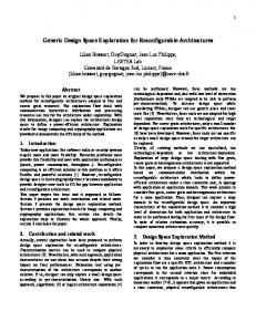
2.1. Grid ALU Processor The main goal of GAP architecture is parallel execution of the program instructions that written sequentially. The GAP combines elements of superscalar processor architectures with a coarsegrained reconfigurable array of functional units [2]. GAP architecture contains a two-dimensional Functional Units (FUs). Instructions are inserted into FUs with Instruction fetch, decode, configuration units, and execute. This processor uses a branch control unit for controlling conditions and ensures correct selection of branches as well as memory access control using load and store units. In addition for faster access to memory it deploys two caches memory which are referred to as instruction cache and data cache. Fetch, decode and configuration units simultaneously work with FUs. The array is arranged in row and columns of ALUs (see the Figure. 1 [2]). Every column in the array is assigned to a single top register in the original GAP architecture. This leads to a number of columns in the array equal to the number of physical registers. Information flow in each column is top to down [1]. Each ALU can read the output information of previous row. ALUs in each row are synchronous and information in a row cannot transfer between ALUs.

24

International Journal of Embedded Systems and Applications (IJESA) Vol.2, No.3, September 2012

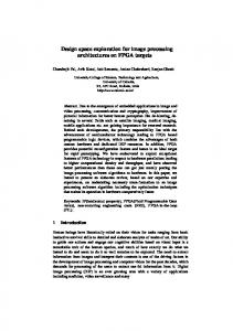
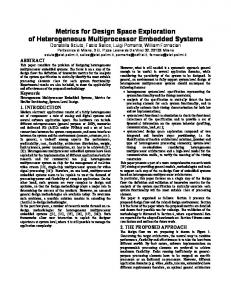
Figure 1. Architecture of the Grid ALU Processor [2] The placement strategy in the ALUs is as follows: instructions that have no dependence on previous instructions (or instructions that related to them) put in a row and execute. Instructions that related to previous instructions can put in to next rows. When facing to a loop, later than placement of loop instructions, in the array for the next iterations of the loop not required to do fetch, decode and configuration steps and instruction can be executed immediately. Branch control unit makes sure misprediction penalty does not occur [1, 14]. The placement of instructions into the array is depicted by the following simple code fragment of pseudo machine instructions that adds 15 numbers out of subsequent memory cells followed by negating the result and depicted in (2). Figure. 2 depicts the dependency graph of the 9 instructions, which can be recognized again at the placement of the instructions within the ALU array shown in fig. 3. The instructions 1 to 3 are placed within the first row of the array. Instruction 4 depends on R2 which is written in the first row and, therefore, it must be located in the second row. It reads the address as a result of instruction 2 and forwards the data received from memory into the column R4 which is the destination register of the load. The instructions 5 to 7 are placed in an analog way. Instruction 8 is a conditional branch that could change program flow. To sustain the hardware simplicity, conditional branches have to be placed below the lowest already arranged instruction. In this case, the branch has to be located after the third row. The last instruction must be placed after the branch in the fourth row. Hence, if the branch is taken, the GAP takes a snapshot of the register contents at the corresponding row and copies the data into the top registers (which is called “Top Regs” in Figure.3). In this case, instruction 9 is discarded. Otherwise, the sub is executed without any time loss [14].

2.2. Multi Objective Optimization To understand, some of the most important concepts are listed below: Multi-objective optimization is a process that usually can make two or more parameters optimal which conflict with each other simultaneously. In most cases where multi optimizations have to be performed there is not a single solution that simultaneously minimizes/maximizes each 25

International Journal of Embedded Systems and Applications (IJESA) Vol.2, No.3, September 2012

objective. Indeed multi-objective optimization would ensure that with changes to one parameter, changes from other parameters do not cause any negative influence on the final result [21]. A general multi-objective problem can be mathematically depicted in equation (1). min/max y = f ( x ) = [f1( x ), f2( x ),…, fm( x )] Subject to: x = x1, x2, …, xn ∈ X y = y1, y2, …, ym ∈ Y

(1)

Where x is called the decision vector, X is the parameter pace, y is the objective vector and Y is the objective space yk = fk(x) where k = 1, 2, 3, …, m. One of the most popular methods that used to solving multi-objective optimization called Pareto Front. Pareto optimality is a concept that formalizes the trade-off between a given set of mutually contradicting objectives. A solution is Pareto optimal when it is not possible to improve one objective without deteriorating at least one of the other. A set of Pareto optimal solutions constitute the Pareto front [21].

3. PROPOSED APPROACH To find an optimal design between possible designs we will use multi-objective optimization based on Pareto Front. The factors that inspect for optimization operation are Clock cycle Per Instruction (CPI) and design complexity. In the section A we talk about calculation of parameters used in optimization process and in section B we explain Pareto Front and how to make use of this method for our approach. 1. 2. 3. 4. 5. 6. 7. 8. 9.

move R1,#15 move R2,#addr move R3,#0 loop: load R4,[R2] add R3,R3,R4 add R2,R2,#4 sub R1,R1,#1 jnz R1,loop ; (end of loop ?) sub R1,R3,R1

(2) 3.1. Calculation of Parameters CPI is a division of CPU clock cycles to count numbers of executed instructions [18]. For calculation of clock cycles, we use a simulator program. We write the simulator in java programming language based on descriptions about GAP that represented in [1, 2, 14, 15, 16]. This simulator would be described in section IV. Parameters that considered for definition of design are: 1) Number of FUs Rows={4, 5, 6,…, 32}, 2) Number of FUs Columns={4, 5, 6,…, 31}, 3) Cache Size={4k, 8k, 16k} and 4) Load/Store Units={Number of Rows}.

26

International Journal of Embedded Systems and Applications (IJESA) Vol.2, No.3, September 2012 1

3

2 move #addr

move #0

move #15

7

4 load

sub #1

8

6

5

add #4

add

jmpnz

9 sub

Figure 2. Dependency graph of the example instructions

Top Regs

R1

R2

R3

R4

0

0

0

0

Load/store

nop 1

move #15

2

move #addr

3

move #0

nop

Branch controller=0?

load 7

sub #1

6

4

add #4

nop

load nop

5 nop

nop

add

nop nop

8 nop

nop

9

sub

nop

Figure 3. Placement of the example instruction Combination of these parameters with different values constructs a set of all possible designs. After constructing the desired set, with execution of a program on simulator, the value of CPI calculated for every state. In this case we test JPEG program because of its potential loop-based structure [3], then GAP can execute it in ideal mode. For calculation of design complexity we use (3) [2, 16]: Complexity = CALUs + CLSUs + Ccache

(3) 27

International Journal of Embedded Systems and Applications (IJESA) Vol.2, No.3, September 2012

In (3) CX presents complexity of element X ∈ {ALUs, Load/Store, Cache}. The values of CALUs, CLSUs, Ccache are respectively calculates from (4), (5) and (6). The variables that used here depicted in Table I. CALU = (Cc*hr + Cr*Cc*hALU) + (Cr*Cc*Cl*hl) CLSUs = (Cr*hLSU) + (Cr*Cl*hl) Ccache = Cache Area*hc

(4) (5) (6)

Table 1. Values of Using Constants in Calculation of Complexity Design Variable

Cr

Value {4, 5, 6,…, 31} {4, 5, 6,…, 32}

Cl

1

hr hALU hl

0.02 1 0.02

hLSU

3.50

hc

3 (1/mm2)

Cc

Comments Number of Columns Number of Rows Number of Configuration Layers for FUs array, in this case we used just one layer complexity of Register FU comprising an ALU Configuration Layer for a FU complexity of Load/store Units complexity of Cache

For calculate hr, hALU, hl, hLSU, and hc we used ratio of area size of each components to area size of source component. We consider ALU as source component, and to calculate area size of components we used results of [22] (in this paper authors calculate area and delay for different hardware elements like cache, integer ALU and etc.). For exapmle hr = (average area for register per bit / average area for integer ALU per bit) = (4.06e+4 / 2.41e+6) = 0.017 ≈ 0.02.

3.2. Approach To find optimal design we will use Pareto Front. According to the definition of Pareto Front [17]: We may define optimization criterion in a multi-objective problem on the basis of dominance concept as follows: for two decision vectors X1 and X2, X1 dominates X2 (X1 ≺ X2) if and only if two conditions are satisfied [19]: 1) X1 is not worse than X2 in all objectives. 2) X1 is strictly better than X2, at least in one objective. The decision vector of X ∈ Xf is also called non-dominated in relation to A ⊆ Xf if and only if ∃ a ∈A ∶ X ≺ a holds. X is Pareto optimum if and only if it is non-dominant in relation to Xf. Thus vertex X is regarded as optimum in perspective of being able to improve none of its objectives regardless of making other objective value worse [17]. To reduce the number of comparisons for finding Pareto optimal (with attention to (7) and (8)), instead of comparing each decision vector with total, first we divide decision vectors to sets that contain two members. In each set, decision vectors are compared and dominating vector goes to the next step, if none of the two vectors can dominate each other, two vectors go to the next step. In the next step, the place of decision vectors are randomly changed for comparison and again vectors are compared to each other. The process continues to have finally a set of decision vectors that non-dominate each other. Such set is the answer. This process depicted in (9). Pseudo code in (10) describes Dominate function that used in (9). 28

International Journal of Embedded Systems and Applications (IJESA) Vol.2, No.3, September 2012

X1