Multi-Objective Optimization of Building Envelope ... - Semantic Scholar

ASHRAE and IBPSA-USA SimBuild 2016 Building Performance Modeling Conference Salt Lake City, UT August 8-12, 2016

Multi-Objective Optimization of Building Envelope, Lighting and HVAC Systems Designs Weili Xu1 , Khee Poh Lam1 , Adrian Chong1 , Omer T. Karaguzel1 1 Center for Building Performance and Diagnostics, Carnegie Mellon University, Pittsburgh, PA

ABSTRACT This paper proposes a computational building design support framework. The framework evaluates and optimizes building envelope systems, electrical systems and HVAC systems simultaneously with the assistance of a newly developed EnergyPlus component cost database. The integrated building system evaluation could potentially reveal the trade-offs among different building systems and help clients and design teams a gain better understanding of high performance designs. A case study based on a real office building is presented to demonstrate the effectiveness of this framework. EnergyPlus v8.3 was used as the building performance evaluation tool. The NSGA-II multi-objective optimization algorithm was employed for acquiring the best design combinations. Results obtained from the optimization process proved that buildings with high performance components will present savings for both first and operation costs. Trade-offs between the first cost and operation costs for different designs were also discussed within five selected optimized cases.

INTRODUCTION The building industry is notoriously driven by the first cost. Life cycle cost analysis (LCCA) might change the design decision-making by forcing the consideration of the net present value of long-term operation costs However, this type of analysis does not usually reveal the tradeoffs between short-term investment and long-term savings, which are important economic details for building stakeholders. To further enhance the process of design decision making, multi-objective building system design optimization, that minimizes first and operation costs simultaneously at the whole building level, could be an effective approach. However, several challenges exist for this approach. One of them is to develop a first cost estimation methodology. Currently, two approaches are frequently employed in research and industry projects. They are the comparative cost estimation method and the quantity take-off (QTO) method. Comparative cost estimation evaluates a project’s costs based on its type, size, location, etc. Machine learning techniques are employed in this method as cost pre-

dictors. However, such an approach is commonly used at the early design stage when only a conceptual design is available (Gunnaydin and Dogan 2004). Unlike comparative cost estimation, QTO can be adopted at most of the design stages. This cost estimation technique focuses on measuring a building’s schematics or work results, which is collected in the bill of quantities (Monteiro and Martins 2013). However, traditional QTO requires manual measurement building components from 2D drawings, which is labor intensive and error-prone. With the growth of Building Information Modeling (BIM) techniques, 3D based BIM-QTO is becoming a preferred process, which offers quick and accurate project cost estimation (Eastman et al. 2011). Despite its popularity, this process is also facing huge challenges. A survey conducted in 2011 indicate that more than 80% of BIM models received by general contractors do not contain adequate data for performing high quality cost estimation (Sattineni and Bradford 2011). The omission of important information will certainly jeopardize the BIM-QTO automation process and force quantity surveyors to move back to the manual process. In addition, it is impossible to calculate building operation costs in this process without integrating building energy simulations. Recent studies propose methods that couple multiobjective optimization with building energy simulation to evaluate project economic impacts (Evins 2013). These methods utilize the computational power of building energy models to estimate both building energy performance profiles and long-term economic impacts. However, some of these studies focus on optimizing a specific system’s performance with regard to a single or multiple objectives. Under such conditions, the optimized system could likely become sub-optimal when integrated with other systems due to the lack of a synergistic relationship between different building systems. On the other hand, studies following a holistic approach for optimizing design parameters usually fix the HVAC system type as a constant input or a set of workarounds is implemented to incorporate HVAC impact on the model response. By fixing the HVAC system type, numerical optimization can only take into account some typical component performance parameters such as chiller COPs or boiler thermal efficiencies.

© 2016 ASHRAE (www.ashrae.org). For personal use only. Additional reproduction, distribution, or transmission in either print or digital form is not permitted without ASHRAE's prior written permission.

110

Such an isolated optimization approach could possibly result in unrealistic product parameters that a designer can never find in the actual product lines of the market. In addition, workaround approaches can lead to inaccurate performance evaluations. This paper presents a method to optimize both first and operation costs of building designs simultaneously with respect to building envelope, electrical lighting and HVAC system design options. A newly developed HVAC autogeneration engine is incorporated in this method to vary HVAC system types during optimization runtime. In addition, the new engine can automatically size system capacities based on energy model settings and design day data. With these two features, the method provides realistic cost estimations for the integrated building systems as well as maintenance and replacement schedules. By considering the interactions between building envelope, lighting and HVAC systems, the whole building simulation can reveal relationships among different design categories thus providing designers a better understanding of their design proposals and return on investment. EnergyPlus is used as the energy simulation engine. A JAVAbased application is introduced to link the building system data, generate EnergyPlus HVAC systems and to perform the NSGA-II optimization algorithm with the use of the JMetal package (Durillo and Nebro 2011).

METHOD Figure 2 shows an overview of the design support framework. The framework consists of five main models namely Building Energy Model (BEM), EnergyPlus HVAC auto generation module, Construction Classification Model (CCM), Cost Optimization Model and BEMQTO Mapping Model. The BEM-QTO Mapping Module is developed to map BEM and CCM for building component cost selection. The additional inputs to this framework are design options, which contain user selected design alternatives for the building, and life cycle cost model. The life cycle cost model carries economic evaluation parameters such as interest rate, price escalation rate, tax rate etc.

EnergyPlus allows building owners and designers holistically appraise different design alternatives for their energy and operation costs. In this framework, a building energy model in EnergyPlus provides building system information to the BEM-QTO Mapping Module for cost mapping. It also computes the whole building life cycle cost once the cost estimation process is completed. HVAC Auto-generation Model Due to the complexity of HVAC system modeling in EnergyPlus, a HVAC auto-generation engine is achieved by a newly developed thermal zone name convention, a HVAC XML data schema and an idf translator that translates XML data into .idf format. The zone name convention and HVAC XML data schema will be detailed in the following sections. Zone Name In a building energy model, thermal zone names should be designed to carry both architectural and HVAC system information. A new naming convention is proposed that allows tools to identify each thermal zone properly. Five elements are required in a zone’s name (Figure 1). They are block, zone function, zone identification, zone’s mechanical ventilation group and its thermal condition group. The first three elements store a zone’s architectural information and the last two elements indicate a zone’s HVAC system information. For instance, Floor6%Office%601%DOAS6%VRF6E2 indicates the number 601 thermal zone is located on the 6th floor and it is an office room. Regarding to its mechanical system information, this zone belongs to the DOAS6 zone group for mechanical ventilation and the VRF6E2 zone group for indoor thermal condition. There are some reserved characters for the last two elements, which are designed for the zones that require special mechanical conditions. For example, an ”EXT” in the ventilation group element means an exhaust system is required in this zone. This zone name convention allows tools to quickly con-

Building Energy Model In the proposed optimization framework, BEM is based on EnergyPlus V8.3 and contains not only building construction and building electric systems, but also HVAC systems. EnergyPlus is one of the advanced whole building simulation engines. It includes comprehensive building components’ descriptions regarding building envelope, electrical and HVAC systems. In addition, its life cycle cost model is well-developed and tested by the Pacific Northwest National Laboratory (PNNL) based on the National Institute of Standards and Technology (NIST) Handbook 135 standard (Cho et al. 2011). Therefore,

Figure 1: Zone Naming Convention struct basic zone activity assumptions and some common HVAC systems. The current tested HVAC systems range from packaged terminal air conditioner, variable air volume (VAV) systems, to hybrid dedicated outdoor air system (DOAS) and variable refrigerant flow (VRF) systems etc.

© 2016 ASHRAE (www.ashrae.org). For personal use only. Additional reproduction, distribution, or transmission in either print or digital form is not permitted without ASHRAE's prior written permission.

111

Figure 2: BEM-QTO Design Decision Support Framework HVAC Data Structure The HVAC data is stored in an XML format. The design of this XML data schema focuses on providing quick data conversion between EnergyPlus .idf data structures and HVAC performance data structures. The design quality attributes of the HVAC system XML data schema includes: 1. Adaptable to common HVAC systems’ performance data 2. Extensible and easy to modify with EnergyPlus version upgrades. The XML format has elements include: : dataset is the parent element that contains the entire data of one specific HVAC system. It has two attributes: 1. setname: specify the HVAC product name of this dataset 2. version: specify EnergyPlus version for this dataset Example: . : object is a child of element. This element represents the objects in EnergyPlus. It has two attributes:

1. description: the name of the EnergyPlus object 2. reference: the object reference. This attribute indicates the sub-system that this object belongs to. Example: . : field is a child element of . This element represents the individual field under an object in EnergyPlus. It also has two attributes: 1. description: the key of a field 2. type: data type, this includes “String”, “Double” and “Integer”. Example: 3.2. The data schema can directly link to the EnergyPlus HVAC system model based on a two-layer logic process. The first layer identifies HVAC system type and EnergyPlus version to extract the corresponding dataset at dataset element. The next step applies auto generation strategies to different sub-systems. For instance, the supply side system is created by analyzing both the ventilation group, and the thermal condition group in the zone name.

© 2016 ASHRAE (www.ashrae.org). For personal use only. Additional reproduction, distribution, or transmission in either print or digital form is not permitted without ASHRAE's prior written permission.

112

Construction Classification Model In Figure 2, the structure of CCM is programmed based on the MasterFormat 2004 classification standard. MasterFormat is one of the leading trade-based industry classification standards developed for construction work that are specified jointly by the Construction Specifications Institute (CSI) and the Construction Specifications Canada (CSC). The classification standard has a 50-year history in the industry, and gained the most recognition for organizing commercial construction specifications in the North American region (CSI and CSC 2005). More importantly, several construction cost data providers such as R RSMeans adopt this standard for constructing their cost database (Gulledge et al. 2007) (Keady 2013). Therefore, in this study, the cost data structure is developed according to MasterFormat 2004 classification and cost data is extracted from RSMeans Building Construction Cost Data (RSMeans 2015). The developed cost model firstly accepts building component specifications from the BEM-QTO Mapping Module, and performs the cost mapping to its database. The mapped cost vector (including material, labor, equipment, total) is then sent back to the BEM-QTO Mapping process for cost estimation.

rithms, the NSGA-II is selected in this study. This algorithm is a well-recognized nondominated sorting based algorithm. It is designed to improve its predecessor’s performance speed while keeping the diversity of the optimal solutions set. It also shows the ability to converge near to the true pareto-optimal front (Deb et al. 2002). The algorithm has been tested on nine different problems. The results demonstrated that the NSGA-II is more effective than the pareto-archived evolution strategy (PAES) and the strength-pareto evolutionary algorithm (SPEA) on most of these problems. Due to its superior performance, the NSGA-II is collected in the JMetal package, a Java based multi-objective optimization framework (Durillo and Nebro 2011). By accessing the JMetal’s API, the BEM-QTO framework could utilize the power of the NSGA-II algorithm to evaluate different design options and form a set of optimal solutions. In the BEM-QTO framework, the building system design problem can be formulated as a multi-objective optimization problem with discrete type parameters: min { f1 (x), f2 (x)}

(1)

Where f1 (x) is the operation costs, which is stated: f1 (x) = xrep − xres + xe + xom&r

(2)

BEM-QTO Mapping Module The BEM-QTO Mapping process is developed for automating the first cost estimation. This process is made of a BEM-QTO mapping system, which implements a data communication protocol to unify both CCM and BEM models’ semantic, and a products cost selection module, to achieve two major objectives respectively: 1. Ensuring a seamless data mapping flow among models; 2. Ensuring the selected building products and their costs are real and available. The mapping system consists of three building system libraries: building envelope system, building HVAC system and building electrical system. The libraries are designed to include EnergyPlus data schema as well as cost mapping elements required for first cost estimation. In addition, each building component can be linked to its own maintenance, repair and replacement (MRR) items in the database. The MRR data will then be exported to EnergyPlus LifeCycleCost:RecurringCosts object for life cycle cost analysis. More information about this object can be found in the EnergyPlus Input/Output reference (LBNL 2013). Optimization The framework focuses on design decision support from the economic perspective of the project. Therefore, first and operation costs are identified as the study objectives and evaluated in a multi-objective optimization process. Among the popular multi-objective optimization algo-

f2 (x) is the first cost and it can be formulated as: f2 (x) = xci + xhi + xei + xrest

(3)

Where xi (first cost), xci (envelope costs), xhi (HVAC system costs), xei (electrical system costs), xrest (other costs), xrep (present value of capital replacement costs), xres (present value of residual value less the disposal costs), xe (present value of energy costs), xom&r (present value of non-fuel operating, maintenance and repair costs). Equation 2 and 3 are adapted from NIST Handbook 135 with no water cost included (Fuller and Petersen 1995).The constraint of this optimization process is:  X = x ∈ Zsc |xi j , i ∈ {1..c} , j ∈ {1..s} (4) The Zsc is the constraint set, which contains the predefined building system types (s) and their cost information (c). The design parameter (x) is specified as discrete independent variables that can only take the values from Zsc .

CASE STUDY The building selected for this study is an office building located in Pittsburgh, Pennsylvania. It consists of four floors, a penthouse floor and a basement with a total of 3700 m2 floor area. The building’s energy model is built in DesignBuilder v4.5 and exported to EnergyPlus v8.3. Figure 3 below shows the geometry of this building as represented in EnergyPlus .dxf file.

© 2016 ASHRAE (www.ashrae.org). For personal use only. Additional reproduction, distribution, or transmission in either print or digital form is not permitted without ASHRAE's prior written permission.

113

Table 2: Life Cycle Cost Model Parameters Field Input Discounting Convention End of Year Inflation Approach Constant Dollar Real Discount Rate 0.03 Base Date 2015 January Service Date 2017 January Study Length 25 Years Tax Rate 0.06 Depreciation Method StraightLine-27 Years Price Escalation NIST Handbook 135 Table Ca-1, Census Region 1 Electricity Tariff Duquesne Light Rate GS Natural Gas Tariff Equitable Gas Rate GSS

Figure 3: Representation of Building in EnergyPlus

Table 1: NSGA-II Parameter Values Parameter Value Crossover SinglePointCrossOver: 90% probability Mutation BitFlipMutation: 17% probability Selection BinaryTournament2 (Deb et al. 2002) Population 30 Maximum Evaluation 900

Besides HVAC systems, there are five other design options, namely external wall and roof constructions, window systems, lighting fixtures and daylighting control options. External wall and roof constructions are built according to Table 16 and 17 in ASHRAE Handbook 2009 Chapter 18 (ASHRAE 2009). Six window system designs are created in WINDOW 6.3 (Table 3). These design options vary from low performance double layer window to high performance quadruple window. Lighting design options contain not only the typical T5, T8 fluorescent lighting fixtures, but also LEDs. Furthermore, occupancy control is also introduced in the evaluation (Table 3). In total, there are 71,820 possible design combinations in this study. A desktop with configuration of i7 quad-core 3.5 GHz CPU and 16 GB RAM is used in this study. Each EnergyPlus simulation takes about 8 minutes. A bruteforce search approach would require more than 400 days to complete a full evaluations. Study Assumptions

Design Variables The designed mechanical conditioning in this building is supplied via 3 air handling units (AHU) and four-pipe fan coil units located within each room. AHU 1 is a VAV system that supplies conditioned air to the basement and first floor through terminal units with reheat coil. AHU 2 is a VAV system that supplies conditioned air only to the auditorium. AHU 3 supplies ventilation to the 2nd, 3rd and 4th floors. Heating and cooling for 2nd, 3rd and 4th floors are provided via a four-pipe fan coil system. Besides the designed VAV system, VRF, and hybrid DOAS and VRF system are also introduced as possible design options for this building. In the design evaluation, the other two HVAC systems’ configurations are kept identical to the designed VAV system.

Compare to brute-force search approach, the optimization algorithm implemented in the framework can greatly reduce the total evaluation time down to a reasonable level. The set up of the NSGA-II can be found in Table 1. The probability of crossover operation is set to the JMetal package, NSGA-II default value. Mutation probability is calculated by 1/N where N is the number of design variables. Each generation evaluates 30 design solutions and the maximum number of evaluation is limited to 900. In total, there are 30 generations in the optimization process. Parallel processing strategy is applied in this framework, which allows computer to evaluate 6 energy simulations concurrently. This strategy could greatly reduce the time required for finding the best design solutions. The total evaluation time takes about 23 hours. Table 2 indicates the parameters used in the life cycle cost

© 2016 ASHRAE (www.ashrae.org). For personal use only. Additional reproduction, distribution, or transmission in either print or digital form is not permitted without ASHRAE's prior written permission.

114

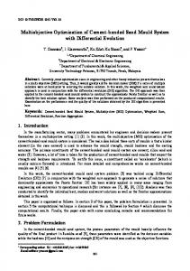
model. These parameters are defined according to the annual supplement report of NIST Handbook 135 (Rushing, Kneifel, and Lavappa 2015). As part of the life cycle cost component, a utility cost model is built based on the local utility provider’s tariff. Unlike average energy cost ($/kWh), the utility cost model can effectively capture the impact of energy demand in different designs. In EnergyPlus, it can accurately identify the cost tariff based on building peak demand for placing excessive energy demand charges ($/kW). This implies that not only a building energy consumption, but also its peak demand, could affect the building’s operation costs. Results and Discussion Figure 4 shows the design solutions’ distribution from the optimization process. The red dots indicate solutions generated at initial generation and purple dots show the solutions generated at last generation. The X-axis is the operations costs of the project and the Y-axis is the first cost of the project. Both of the costs are valued in USD ($). At initial stage, a wide dispersion of red dots suggest that the the NSGA-II algorithm are exploring the entire solution space. As the process continues, the design cases are slowly converging to the region at the lower left corner of the solution space, which shows lower first and operation costs. The adequacy of 900 evaluations is also tested. Figure 5 compares a few selected pareto front curves generated along the optimization process with the final pareto front curve. At the beginning, the pareto front curve at 2nd

First Cost ($)

Figure 4: Distribution of design solutions generated by the NSGA-II process 2500000 2250000 2000000 1750000 1500000

● ●● ● ● ● ● ● ●● ●● ● ● ● ● ●●●● ●●● ● ●● ● ●● ● ● ●● ● ● ●● ● ●● ● ● ●● ●● ●●

1250000 1800000

2000000

Generation

●

● ●

●

2

●

30

●

2200000

Operation Cost ($) First Cost ($)

Table 3: Window and Lighting Design Option Design Property Unit Cost Window: Dou- U-3.13, SHGC- $242.19/m2 ble Clear (DC) 0.73, Vt-0.8 Window: Dou- U-2.58, SHGC- $290.36/m2 ble Tinted (DT) 0.37, Vt-0.53 Window: Dou- U-1.4, SHGC- $356.82/m2 ble Thick Clear 0.41, Vt-0.61 (DTC) Window: Heat U-1.4, SHGC- $478.99/m2 Reflective Clear 0.25, Vt-0.45 (HRC) Window: Triple U-0.81, SHGC- $480.00/m2 Glazing (TG) 0.71, Vt-0.53 Window: U-0.781, SHGC- $862.00/m2 Quadruple (Q) 0.46, Vt-0.62 Light: T8 10.2W /m2 $149.5/m2 2 Light: T5 8W /m $163.5/m2 2 Light: LED 6.5W /m $389.5/m2 Occupancy $268/Each Sensor Note: The unit of U value is W/m2 ◦ C

2000000 1750000 1500000

● ● ● ●● ● ● ● ● ● ●● ● ● ● ● ●

1250000 1800000

1900000

Generation

● ● ●

2000000

●● ●● ●

2100000

●

29

●

30

●

2200000

Operation Cost ($)

Figure 5: Pareto front curves comparison

generation shows a large deviation from the final pareto front curve. As the generation increases, the generated pareto front curves become closer to the final pareto front curve. The lower graph shows a small deviation between the pareto front curve at generation 29 and the final pareto front curve, which shows that the final pareto front curve could be close to the global pareto front curve. Besides solutions generated from optimization, a base case model is created that represents the initial design. The initial design uses design options that have the lowest normalized unit cost. In the final pareto front curve, 30 design options are suggested. Among them, 6 cases are selected for comparison. They are the highest first cost (Case 26), lowest first cost (Case 13), highest operation costs (Case 25), lowest operation cost (Case 4), highest life cycle cost (Case 26) and lowest life cycle cost (Case 1). Table 4 shows the design solutions for each of the selected case and their correspondent first cost as well as operation costs. In Table 4, both base case’s first cost and operation costs are higher than the optimized cases’. For first cost, though the base case model installs all the cheapest design options, its HVAC sizing results suggest a large amount of initial investment on the mechanical system. In

© 2016 ASHRAE (www.ashrae.org). For personal use only. Additional reproduction, distribution, or transmission in either print or digital form is not permitted without ASHRAE's prior written permission.

115

Table 4: Optimal Solution Packages

a: b:

Case

Walla

Roofa

Window Light

Base 1 4 13 25 26

24 9 34 7 22 9

9 3 17 7 16 4

DC TG TG HRC TG TG

T8 LED LED LED T5 LED

Daylight

HVAC

Off On On Off On On

VAV VRF DVb VRF VRF DVb

First Cost ($) 2,286,433 1,309,218 2,114,405 1,260,953 1,287,545 2,181,651

Operation Costs ($) 2,324,763 1,945,480 1,808,939 2,160,938 2,256,787 1,810,763

ABEFC ($) 0 1,356,498 687,852 1,189,305 1,066,864 618,782

Wall and Roof number is based on ASHRAE Handbook 2009 Fundamental Chapter 18 Table 16 and 17. DV denotes hybrid DOAS and VRF system.

addition, due to its lower performance design, base case’s EUI is nearly 60% higher than optimized cases, which lead to higher operation costs. Since all the optimized cases have lower first and operation costs, there is no payback period for the project investment. Therefore, Additional Break-Even First Cost (ABEFC) analysis is used in this study. ABEFC is a first cost based analysis, which converts all the savings in the project period to first cost. With this method, project stakeholders can compare optimized cases by evaluating how much additional first cost could be justified to break even the base case (Mumma 2002). In this study, the ABEFC is equal to the life cycle cost difference between optimized cases and base case. In Table 4, Case 1 is not only the lowest life cycle cost case, but also has the most additional first cost. With almost $1.4 million saved, clients or design teams could invest on high efficiency equipment or design elements that can create a more comfortable working environment. Besides Case 1, other optimized cases also achieve a large amount of additional first cost. Besides the additional first cost, clients and design teams can also compare the trade-offs between first and operation costs among the optimized cases by visualizing the solutions on pareto front curve. Figure 6 shows a possible decision making scenario. The upper graph indicates this project’s first and operation costs can be reduced by 42% and 16% respectively by moving from base case (red dot) to case 25. Trade-offs between optimized cases can also be visualized on the same graph. The lower graph in Figure 6 shows a 4% increase in first cost and 13% decrease in operation costs by changing from case 25 to case 1. By visualizing the results, clients and design teams can adjust their design choice based on project budget and predicted operation period. Table 4 also suggests the most common systems for optimized cases. They are triple glazing, LED, occupancy light control and VRF systems. These systems are the expensive design options; however, they can effectively reduce building energy consumption and building peak demand. A smaller peak demand means a smaller and

Figure 6: Decision making process less complicated HVAC system. If the savings from the HVAC system is significant, the incremental costs from envelope and electrical systems can be minimized, or even reduced. Besides the first cost savings, integrating high performance envelope, electrical and HVAC systems can potentially yield a lower life cycle cost as well.

CONCLUSION A BEM-QTO framework for building systems design decision making is proposed in this study. The following list summarizes the features of this framework: 1. Project budget can be estimated according to the national construction classification using the BEM model 2. With the newly developed HVAC data schema, different HVAC systems can be automatically generated in EnergyPlus according to the predefined ventilation groups and thermal condition groups. 3. The NSGA-II algorithm is demonstrated to be effective in building system design optimization. The

© 2016 ASHRAE (www.ashrae.org). For personal use only. Additional reproduction, distribution, or transmission in either print or digital form is not permitted without ASHRAE's prior written permission.

116

algorithm can find nearly optimal design solutions while greatly reducing the evaluation time. 4. Building life cycle cost analysis can be performed at a integrative level, which not only considers the performance of each individual system, but also the interactions among the building systems. 5. The framework offers design solution packages with consideration of the first cost as well as operation costs for each solution. 6. The generated design solutions are realistic, which can be directly drawn from the results and used for detail cost estimation and the bill of quantities. The current framework is limited to building systems and component evaluation. Therefore, building system control strategies are not considered in this study. This is not only because the cost of system control strategies is difficult to estimate, but also the evaluation requires mixed integer and double data type, which could fundamentally change the behaviors of operators in the NSGA-II algorithm. Further development of this implementation is under progress. In addition, because building energy simulation require extensive computational power, the number of building system design options should be limited to a relatively small set to avoid a large amount of evaluation time. Therefore, expert knowledge is required before performing this method. Lastly, several critical cost components such as ducts and pipes are not considered in the first cost estimation process. This is because BEM does not provide such information in the simulation results. Potential future work could connect this framework with a fully specified Building Information Model, which offers quantity counts for such building elements.

REFERENCES ASHRAE. 2009. ASHRAE Handbook 2009 Fundamental. Atlanta, GA: American Society of Heating, Refrigerating and Air-Conditioning Engineers.

Durillo, Juan J., and Antonio J. Nebro. 2011. “jMetal: A Java framework for multi-objective optimization.” Advances in Engineering Software 42:760–771. Eastman, Chuck, paul Teicholz, Sacks Rafael, and Kathleen Liston. 2011. A BIM Application Areas For Owners. Hoboken, New Jersey: John Wiley & Sons Inc. Evins, Ralph. 2013. “A review of computational optimisation methods applied to sustainable building design.” Renewable and Sustainable Energy Review 22:230–245. Fuller, S K, and S R Petersen. 1995. NIST Handbook 135: Life-Cycle Costing Manual for the Federal Energy Management Program. Gaithersburgh, MD: National Institute of Standards and Technology. Gulledge, Charles E, Lane J Beougher, Michael J King, Robert Paul Dean, Dennis J Hall, Nina M Giglio, G Wade Bevier, and Phil Steinberg. 2007. “MasterFormat 2004 Edition 2007 Implementation Assessment.” Technical Report, Continental Automated Building Association. Gunnaydin, H Murat, and S Zeynep Dogan. 2004. “A neural network approach for early cost estimation of structural systems of buildings.” International Journal of Project Management, p. 595. Keady, R A. 2013. Equipment Inventories for Owners and Facility Managers: Standards, Strategies and Best Practices. Hoboken, New Jersey: John Wiley & Sons Inc. LBNL. 2013. “Input Output Reference: The Encyclopedic Reference to EnergyPlus Input and Output.” Technical Report, Lawrence Berkeley National Laboratory. Monteiro, Andre, and Joao Pocas Martins. 2013. “A survey on modeling guidelines for quantity takeofforiented BIM-based design.” Automation in Construction, pp. 238–253.

Cho, H, W Wang, A Makhmalbaf, K Yun, J Glazer, L Scheier, V Srivastava, and K Gowri. 2011. “Extend EnergyPlus to Support Evaluation, Design, and Operation of Low Energy Buildings.” Technical Report, Pacific Northwest National Laboratory.

Mumma, Stanley A. 2002. “Using Dedicated Outdoor Air Systems: Economics of improved environmental quality.” ASHRAE Journal 1:1–10.

CSI, and CSC. 2005. “MasterFormat TM 2004 Edition Numbers & Tiles.” Technical Report, Construction Specifications Institute and Construction Specifications Canada.

Rushing, Amy S, Joshua D Kneifel, and Priya Lavappa. 2015. “Energy Price Indices and Discount Factors for Life Cycle Cost Analysis 2015.” Technical Report, National Institute of Standards and Technology.

Deb, Kalyanmoy, Amrit Pratap, Sameer Agarwal, and TAMT Meyarivan. 2002. “A fast and elitist multiobjective genetic algorithm: NSGA-II.” Evolutionary Computation, IEEE Transactions on 6 (2): 182–197.

Sattineni, Anoop, and R Harrison Bradford. 2011. “Estimating with BIM: A survey of US Construction Companies.” ISARC Conference, Seoul, Korea.

RSMeans. 2015. Building Construction Cost Data. Norwell, MA: Construction Publishers & Consultants.

© 2016 ASHRAE (www.ashrae.org). For personal use only. Additional reproduction, distribution, or transmission in either print or digital form is not permitted without ASHRAE's prior written permission.

117