Multi-Resolution Image Fusion by FFT - Core

2011 International Conference on Image Information Processing (ICIIP 2011)

Multi-Resolution Image Fusion by FFT VPS Naidu Multi Sensor Data Fusion Lab Flight Mechanics and Control Division CSIR - National Aerospace Laboratories Bangalore, India [email protected]

Abstract— Multi-resolution image analysis by Fast Fourier Transform (MFFT) algorithm has been presented and evaluated for pixel level image fusion. The idea is to apply simple and proven technique of FFT to image fusion. The performance of this algorithm is compared with that of well known wavelet based image fusion technique. It is observed that the performance of image fusion by MFFT is slightly better than wavelet based image fusion algorithm. It is computationally very simple and it could be well suited for real time applications. Keywords- Multi resolution, Image fusion, FFT, image processing, wavelets, fusion quality, fusion rule;

I.

INTRODUCTION

Image fusion has emerged as an innovative and promising research area in recent years. Image fusion has many applications in the areas of military, remote sensing, machine vision, robotic, surveillance and medical imaging etc. The objective of image fusion is to merge the information content from several images (or acquired from different imaging sensors or modalities) taken from the same scene into a single image that contains the finest information coming from the individual source images [1]. Hence, the fused image provides enhanced superiority image than any of the original source images. Depending on the merging stage, image fusion could be performed at three different levels viz. pixel level, feature level and decision level [2,3]. Among these, pixel level image fusion is the simplest method in which the images are fused at sensor level. The simplest pixel level image fusion is to take the average of the grey level source images pixel by pixel. This technique produces fused image with several undesired effects and reduced feature contrast. To overcome these problems, multiresolution algorithms such as wavelets [1,4,5], multi-scale transforms such as image pyramids [3,6,7], spatial frequency [8,9] and fuzzy set theory [10] have been proposed. In multiresolution image fusion (MIF), two or more registered images are combined to increase the spatial resolution of acquired low detail multi-sensor images and preserving their spectral information. Multi-resolution wavelet transforms could provide good localization in both spatial and frequency domains. Discrete wavelet transform would provide directional information in decomposition levels and contain unique information at different resolutions [4, 5]. In this chapter, the multi-resolution image analysis by fast Fourier transform (MFFT) is applied to fuse the source images at pixel level. The idea is to apply simple and proven

technique of FFT to image fusion. One of the important prerequisites to be able to apply fusion techniques on source images is the image registration i.e., the information in the source images needed to be adequately aligned or registered prior to fusion of the images. In this chapter, it is assumed that the source images are already registered. II.

DISCRETE FOURIER TRANSFORM

The 2D discrete Fourier transform X ( k1 , k 2 ) of an image or 2D signal x ( n1 , n2 ) of size N1 xN 2 is defined as:

X (k1 , k2 ) =

1 N2 N2

N1 −1N 2 −1

∑∑

x(n1 , n2 )e

⎛k n k n ⎞ − i 2π ⎜⎜ 1 1 + 2 2 ⎟⎟ N2 ⎠ ⎝ N1

n1 = 0 n 2 = 0

where 0 ≤ k1 ≤ N1 − 1 and 0 ≤ k 2 ≤ N 2 − 1 (1) Similarly, the 2D inverse discrete Fourier transform is defined as:

x (n1 , n 2 ) =

N 1 −1 N 2 − 1

∑∑

X ( k 1 , k 2 )e

⎛k n k n ⎞ i 2 π ⎜⎜ 1 1 + 2 2 ⎟⎟ N2 ⎠ ⎝ N1

n1 = 0 n 2 = 0

where 0 ≤ n1 ≤ N 1 − 1 and 0 ≤ n 2 ≤ N 2 − 1 (2) Both DFT and IDFT are separable transformations and the advantage of this property is that 2D DFT or 2D IDFT can be computed in two steps by successive 1D DFT or 1D IDFT operations on columns followed by the resulting rows (or vice versa) of an image x ( n1 , n2 ) as shown in eq.3 [11-16]. DFT is more complex and to overcome this, one can employ fast Fourier transform (FFT).

1 X (k1 , k 2 ) = N2 N2 III.

⎛kn ⎞ ⎛k n ⎞ ⎡ −i 2π ⎜⎜ 1 1 ⎟⎟ ⎤ −i 2π ⎜⎜ 2 2 ⎟⎟ N1 ⎠ ⎝ ⎢ ∑ x(n1 , n2 )e ⎥e ⎝ N 2 ⎠ (3) ∑ ⎢ ⎥ n2 = 0 n1 = 0 ⎣ ⎦ N 2 −1 N1 −1

MULTI-RESOLUTION ANALYSIS

Multi-resolution image analysis by fast Fourier transform (MFFT) is very much similar to wavelets transform, where signal is filtered separately by low pass and high pass finite impulse response (FIR) filters and the output of each filter is decimated by a factor of two to achieve first level of decomposition. The decimated low pass filtered output is filtered again separately by low pass and high pass filter followed by decimation by a factor of two provides second level of decomposition. The successive levels of decomposition can be achieved by repeating this procedure.

Proceedings of the 2011 International Conference on Image Information Processing (ICIIP 2011)

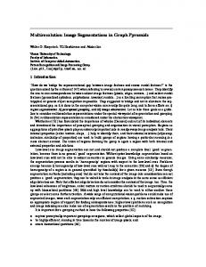
2011 International Conference on Image Information Processing (ICIIP 2011) The idea behind the MFFT is to replace the FIR filters with FFT. The information flow diagram of MFFT (one level of decomposition) is shown in Fig-1 [17]. The image to be decomposed is transformed into frequency domain by applying FFT in column wise. Take IFFT on first 50% of points (0 to 0.5π ) to get the low passed image L . Similarly, take IFFT on second 50% of points ( 0.5π to π ) to get the high passed image H . The low passed image L is transformed into frequency domain by applying FFT in row wise. Take IFFT on first 50% of points (in row wise) to get low passed image LL and similarly take IFFT on the remaining 50% to get the lowhigh passed image LH . The high passed image H is transformed into frequency domain by applying FFT in row wise. Take IFFT on first 50% of points (in row wise) to get high-low passed image HL and similarly take IFFT on the remaining 50% to get the high passed image HH . The low passed image LL contains the average image information corresponding to low frequency band of multi scale decomposition. It could be considered as smoothed and sub sampled version of the source image. It represents the approximation of source image. LH , HL and HH are detailed sub images which contain directional (horizontal, vertical and diagonal) information of the source image due to spatial orientation. Multi resolution could be achieved by recursively a/c : along columns a/r : along rows

Image

Fig. 2a Ground truth image

applying the same algorithm to low pass coefficients ( LL ) from the previous decomposition. Image can be reconstructed by reversing the above outlined procedure. The ground truth (reference) image used in multiresolution analysis is shown in Fig-2a. First and second levels of decomposition of Fig-2a are shown in Fig-2b. The reconstructed image from 2nd level of decomposition is shown in Fig-2c. One can observed from this figure that the reconstructed image is exactly matched with the ground truth image. It means that there is no information loss with this analysis. It is known that wavelet method trades spatial resolution to frequency resolution at different scales. There is no trade-off between spatial and frequency resolution, when FFT is considered on whole image. Trade-off between spatial and frequency resolution can be obtained using the MFFT at different scales of decomposition instead of applying FFT on entire image.

FFT a/r

0.5π

0

L

π IFFT a/r

H

i)

First level of decomposition

FFT a/c

0

LL

LH

HL HH π

ii) Second level of decomposition Fig. 2b Multi resolution image decomposition

IFFT a/c Fig. 1 Multi-resolution decomposition structures

Proceedings of the 2011 International Conference on Image Information Processing (ICIIP 2011)

2011 International Conference on Image Information Processing (ICIIP 2011) into D levels using MFFT. The resultent decomposed images from I 1 and I 2 are [17]

{ { LH , HH , HL } → { LL , { LH , HH , HL }

I 1 → 1 LLD , I2

i)

Reconstructed image

1

1

1

d

2

d

2

2

D

d d =1, 2,..., D

2

d

d

d d =1, 2,..., D

} }

At each decomposition level d ( d = 1,2,..., D ) , the fusion rule will select the larger absolute value of the two MFFT detailed coeficients, since the detailed coeficients are corresponds to sharper brightness changes in the images such as edges and object boundaries etc. These coeficients are fluctuating around zero. At the coarest level ( d = D) , the fusion rule takes average of the MFFT approximation coeficients since the approximation coeficents at coarser level are the smoothed and subsampled verion of the original image. The fused image I f can be obtained using [17] :

If ←

{ LL , { LH , f

f

D

V.

d

f

HH d , f HLd

}

d =1, 2 ,..., D

}

(4)

PERFORMANCE EVALUATION

A. With reference image When the reference image is available, the performance of image fusion algorithms can be evaluated using the following metrics: ii) Error image Fig. 2c Reconstructed image from 2nd level of decomposition and the error image

IV.

FUSION

The information flow diagram of MFFT based pixel level image fusion scheme is shown in Fig-3. One can observe that the modification of the present scheme is the use MFFT instead of wavelets. The images to be fused I 1 and I 2 are decomposed Images to be fused

1.

PFE =

2.

MFFT’s of source images

Fusion rules

MFFT of fused image

norm( I r )

(5)

*100

Peak Signal to Noise Ratio (PSNR) [5,19] ⎛ ⎜ ⎜ PSNR = 20log10 ⎜ 1 ⎜⎜ MN ⎝

⎞ ⎟ L ⎟ M N ⎟ 2 (I r (i, j) − I f (i, j)) ⎟⎟ ∑∑ i =1 j =1 ⎠ 2

B. Without reference image When the reference image is not available, the following metrics could be used to test the performance of the fused algorithms. 1.

Standard Deviation (SD) [5,20] L

L

i =0

i =0

∑ (i − i ) 2 hI f (i) , i = ∑ ihI f

Fused image Fig. 3 Schematic diagram for the MFFT image fusion scheme

(6)

where L in the number of gray levels in the image Its value will be high when the fused and reference images are similar. Higher value implies better fusion.

σ= If

norm( I r − I f )

where norm is the operator to compute the largest singular value It is computed as the norm of the difference between the corresponding pixels of reference and fused images to the norm of the reference image. This will be zero when both reference and fused images are exactly alike and it will be increased when the fused image is deviated from the reference image.

I2

I1

Percentage Fit Error (PFE) [5,18]

Proceedings of the 2011 International Conference on Image Information Processing (ICIIP 2011)

(7)

2011 International Conference on Image Information Processing (ICIIP 2011) where

hI f (i) is the normalized histogram of the fused

image I f ( x, y) and L number of frequency bins in the histogram. It is known that standard deviation is composed of the signal and noise parts. This metric would be more efficient in the absence of noise. It measures the contrast in the fused image. An image with high contrast would have a high standard deviation. 2.

Spatial Frequency (SF) [5,8,9] Spatial frequency criterion is: SF = RF 2 + CF 2 (8) where row frequency of the image: RF =

1 MN

M

N

∑∑ [ I

f

(a)

Reference image I r

( x, y ) − I f ( x, y − 1)] 2

x =1 y = 2

column frequency of the image: CF =

1 MN

N

M

∑ ∑ [I

f

( x , y ) − I f ( x − 1, y )] 2

y =1 x = 2

This frequency in spatial domain indicates the overall activity level in the fused image. ( x, y ) is the pixel index. The fused image with high SF would be considered. VI.

RESULTS AND DISCUSSION

NAL’s indigenous aircraft SARAS, shown in Fig-4a [17], is considered as a reference (ground truth) image to evaluate the performance of the proposed fusion algorithm. The complimentary pair input images (data set-1) are taken to evaluate the fusion algorithm and these images are shown in Fig-4b and Fig-4c. The complementary pair has been created by blurring the reference image of size 512 x 512 with a Gaussian mask using diameter of 12 pixels. The images are complementary in the sense that the blurring occurs at the top half and the bottom half respectively. The first column in Fig5 to Fig-6 shows fused images and the second column shows the error images. The error (difference) image is computed by taking the corresponding pixel difference of reference image I ( x, y ) = I ( x, y ) − I ( x, y )

r f . The fused and and fused image i.e. e error images by one level of decomposition using MFFT and wavelet fusion algorithms are shown in Fig-5 and Fig-6 respectively. Similarly the fused images by two levels of decomposition using MFFT (1st column) and wavelet (2nd column) [5] are shown in Fig-7. It is observed that the fused images of both MFFT and wavelets are almost similar for these images. The reason could be because of taking the complementary pairs. One can observe that the fused image preserves all the useful information from the two source images. The performance metrics for evaluating the image fusion algorithms are shown in Table-1. The metrics showed in table in bold font are better among others. From the table it is observed that MFFT with higher level of decomposition performed well. In second data set, forward looking infrared (FLIR) image (1st column) and low light television (LLTV) image (2nd column) are considered for evaluation of the fusion algorithms (data set-2) and are shown in Fig-8 [21]. Roads appear very clear in FLIR image since the roads are high thermal contrast. Trees and light spots appear in LLTV image.

(b) First source image I 1

(c) Second source image I 2 Fig. 4 Reference and source images

The fused images by MFFT (1st column) and wavelets (2nd column) are shown in Fig-9. The fused image preserves all the useful information from the LLTV and FLIR images. The fusion performance metrics are shown in Table-I. It is observed that fusion by MFFT shows better performance than wavelets. From the results, one can observe that the fused or combined image containing the truthful description or information than individual source images. Higher level of decomposition used in fusion process gives better performance. Fusion by MFFT with higher level of decomposition showed small PFE and high PSNR that shows the fused image is very similar to the ground truth image. Similarly, SD and SF are high that shows that the fused image having good contrast and retain the overall activity. VII. CONCLUDING REMARKS Multi-resolution image analysis by Fast Fourier Transform (MFFT) algorithm has been presented and evaluated for pixel level image fusion. The idea is to apply simple and proven

Proceedings of the 2011 International Conference on Image Information Processing (ICIIP 2011)

2011 International Conference on Image Information Processing (ICIIP 2011) technique of FFT to image fusion. The performance of this algorithm is compared with well known wavelets based image fusion technique. It is computationally very simple and it could be well suited for real time applications. It is observed that image fusion by MFFT perform slightly better than wavelet based image fusion algorithm. This algorithm can be used to fuse multi-aspect images as well. Different orientation images should be registered before fuse them. If the source images are different sizes (resolutions), decompose the images into different levels and wherever the sizes match, then fuse them. If one of the source images is color and other is gray image, then convert the color image into gray and then fusion can be done. REFERENCES [1] [2] [3]

[4]

[5]

[6]

Gonzalo Pajares and Jesus Manuel de la Cruz, “A wavelet-based image fusion tutorial”, Pattern Recognition, 37, 2007, pp.1855-1872. Varsheny P.K., “Multisensor data fusion”, Elec. Comm. Engg., Journal, Vol9 (12), pp. 245-253, 1997. P.J. Burt and R.J. Lolczynski, “Enhanced image capture through fusion”, In Proc. The 4th Int. Conf. on Computer Vision, pp. 173-182, Berlin, Germany, 1993. S.G. Mallet, “A theory for multiresolution signal decomposition: The wavelet representation”, IEEE Trans. Pattern Anal. Mach. Intel., Vol. 11(7), pp. 674-693, 1989. VPS Naidu and J.R. Raol, ”Pixel-Level Image Fusion using Wavelets and Principal Component Analysis – A Comparative Analysis” Defence Science Journal, Vol.58, No.3, pp.338-352, May 2008. F. Jahard, D.A. Fish, A.A. Rio and C.P. Thompson, “Far/near infrared adapted pyramid-based fusion for automotive night vision”, IEEE Proc. 6th Int. Conf. on Image Processing and its Applications (IPA97), pp.886890, 1997. Levels of decomposition

D =1 D =1

D=2 D=2

[7]

[8]

[9]

[10] [11] [12] [13] [14] [15]

[16] [17] [18]

[19] [20] [21]

B. Ajazzi, L. Alparone, S. Baronti and R. Carla, “Assessment pyramidbased multisensor image data fusion”, Proc. SPIE 3500, pp.237-248, 1998. Shutao Li, James T. Kwok and Yaonan Wang, “Combination of images with diverse focuses using the spatial frequency”, Information fusion, 2(3), pp.167-176, 2001. VPS Naidu and J.R. Raol, “Fusion of Out Of Focus Images using Principal Component Analysis and Spatial Frequency”, Journal of Aerospace Sciences and Technologies, Vol. 60, No. 3, pp.216-225, Aug. 2008. Abdilhossein Nejatali and L.R. Ciric, “Novel image fusion methodology using fuzzy set theory”, Opt. Eng., 37(2), pp.485-491, 1998. http://www.cs.toronto.edu/~fleet/courses/D71/winter09/Handouts/fourier 2D.pdf R.C. Gonzalez and P. Wintz, “Digital Image Processing”, MA: AddisonWesley, 1987. http://morse.cs.byu.edu/450/lectures/lect18/ft-2d.slides.printing.6.pdf http://www.cs.unm.edu/~williams/cs530/ft2d.pdf12 [27] Andew B. Watson and Allen Poirson, “Separable two-dimensional discrete Hartly transform”, J. opt. Soc. Am. A, Vol.3, No.12, pp.200104, Dec. 1986. http://homepages.inf.ed.ac.uk/rbf/HIPR2/fourier.htm VPS Naidu, “Discrete Cosine Transform-based Image Fusion”, Defence Science Journal, Vol. 60, No.1, pp.48-54, Jan.2010. VPS Naidu, Girija G. and J.R. Raol, “Evaluation of data association and fusion algorithms for tracking in the presence of measurement loss”, AIAA Conference on Navigation, Guidance and Control, Austin, USA, 11-14, August 2003. Gonzalo R. Arce, “Nonlinear Signal Processing – A statistical approach”, Wiley-Interscience Inc., Publication, USA, 2005. Rick S. Blum and Zheng Liu, “Multi-sensor image fusion and its applications”, CRC Press, Taylor & Francis Group, NW, 2006. http://www.imagefusion.org

TABLE I: PERFORMANCE EVALUATION METRICS algorithm Data set-1 With reference Without reference PFE PSNR SD SF MFFT 2.719 40.145 49.291 15.066 wavelets 3.789 38.703 46.232 13.084 MFFT 2.675 40.217 49.344 15.748 wavelets 3.203 39.434 46.995 15.698

Data set-2 Without reference SD SF 59.7 38 47.83 14.97 59.77 38.25 48.56 17.11

Fig. 5 Fused (1st column) and error (2nd column) image with one level ( D = 1) of decomposition using MFFT – data set-1

Proceedings of the 2011 International Conference on Image Information Processing (ICIIP 2011)

2011 International Conference on Image Information Processing (ICIIP 2011)

Fig. 6 Fused (1st column) and error (2nd column) image with one level ( D = 1) of decomposition using wavelets – data set-1

Fig. 7 Fused images with two levels of decomposition using MFFT (1st column) and wavelets (2nd column) – data set-1

Fig. 8 FLIR (1st column) and LLTV (2nd column) images – data set-2

Fig. 9 Fused images with two levels ( D = 2) of decomposition using MFFT (1st column) and wavelets (2nd column) – data set-2

Proceedings of the 2011 International Conference on Image Information Processing (ICIIP 2011)