Multi-Task Learning with Neural Networks for Voice Query ...

Multi-Task Learning with Neural Networks for Voice Query Understanding on an Entertainment Platform Jinfeng Rao,1,2 Ferhan Ture,1 and Jimmy Lin3 1

Comcast Applied AI Research Lab Department of Computer Science, University of Maryland 3 David R. Cheriton School of Computer Science, University of Waterloo [email protected],[email protected],[email protected] 2

ABSTRACT We tackle the challenge of understanding voice queries posed against the Comcast Xfinity X1 entertainment platform, where consumers direct speech input at their “voice remotes”. Such queries range from specific program navigation (i.e., watch a movie) to requests with vague intents and even queries that have nothing to do with watching TV. We present successively richer neural network architectures to tackle this challenge based on two key insights: The first is that session context can be exploited to disambiguate queries and recover from ASR errors, which we operationalize with hierarchical recurrent neural networks. The second insight is that query understanding requires evidence integration across multiple related tasks, which we identify as program prediction, intent classification, and query tagging. We present a novel multi-task neural architecture that jointly learns to accomplish all three tasks. Our initial model, already deployed in production, serves millions of queries daily with an improved customer experience. The novel multi-task learning model, first described here, is evaluated through carefully-controlled laboratory experiments, which demonstrates further gains in effectiveness and increased system capabilities. ACM Reference Format: Jinfeng Rao, Ferhan Ture, and Jimmy Lin. 2018. Multi-Task Learning with Neural Networks for Voice Query Understanding on an Entertainment Platform. In KDD 2018: 24th ACM SIGKDD International Conference on Knowledge Discovery & Data Mining, August 19–23, 2018, London, United Kingdom. ACM, New York, NY, USA, 10 pages. https://doi.org/10.1145/3219819.3219870

1

INTRODUCTION

In recent years, we have witnessed a proliferation of smart home gadgets and speech-driven intelligent agents such as Amazon Alexa and Google Home. It is only natural that viewers should be able to engage with their home entertainment systems (i.e., TVs) in a similar manner, via natural speech-based interactions. The Comcast Xfinity X1 entertainment platform provides this capability. At a high level, our goal is simple—we want to provide the most natural speech-based interactions with TVs possible. The viewer issues a voice query, our platform understands the intent, and then Permission to make digital or hard copies of all or part of this work for personal or classroom use is granted without fee provided that copies are not made or distributed for profit or commercial advantage and that copies bear this notice and the full citation on the first page. Copyrights for components of this work owned by others than the author(s) must be honored. Abstracting with credit is permitted. To copy otherwise, or republish, to post on servers or to redistribute to lists, requires prior specific permission and/or a fee. Request permissions from [email protected]. KDD 2018, August 19–23, 2018, London, United Kingdom © 2018 Copyright held by the owner/author(s). Publication rights licensed to ACM. ACM ISBN 978-1-4503-5552-0/18/08. . . $15.00 https://doi.org/10.1145/3219819.3219870

responds appropriately. For example, the viewer simply says “watch Inception on demand” to switch the television to the proper listing, which is much simpler than awkwardly going through channel guides or spelling out the name of the movie on a keypad. Even if the viewer already knows what channel a program is on, finding the right channel may still be difficult, since modern entertainment packages may have hundreds of channels. Our query logs suggest that the voice query functionality receives significant usage, and has emerged as an attractive alternative to physical button entry on remote controls that have gotten too complex over time. Our first attempt at tackling this challenge focused on directly identifying the program a viewer intends to watch, what we term voice query navigation. The key insight is to exploit session context to disambiguate queries and to cope with speech recognition errors. For example, the query “game of throw” can either refer to the television series “Game of Thrones” (because of a transcription error) or a TV game called “Fish Throw Game". However, if the viewer just uttered “HBO series” a moment ago, then it is far more likely that she is looking for the former since we know the show is playing on HBO. This intuition is operationalized using a Navigational Hierarchical Recurrent Neural Network (N-HRNN), previously described in Rao et al. [24]. Our N-HRNN was recently deployed into production to serve live traffic at the tail end of a cascade architecture, as part of a riskaverse deployment strategy. At present, the model serves millions of queries daily for which the previous modules provide no response (in other words, the most difficult queries). We have substantially increased end-to-end coverage, reducing the number of unhandled queries by three quarters. On these queries, the N-HRNN definitively improved the customer experience two thirds of the time and arguably did not hurt in the other third. Despite the success of our N-HRNN in production, we noticed two main shortcomings. First, the model adopts a classificationbased approach, which is unable to predict unseen programs (e.g., newly-added content). Furthermore, its formulation has difficulty handling the long tail of rarely-watched programs. Second, our analysis of millions of queries [25] reveals that they span the gamut from program navigation to vague entertainment intents (e.g., looking for kids cartoons) to direct commands (e.g., turning on closed captioning) to queries that have nothing to do with entertainment (e.g., checking the weather). In fact, we find that around 40% of queries are either ambiguous viewing intents or not related to viewing a program at all. Obviously, a model based on program prediction cannot handle such queries. These two main shortcomings motivated us to explore a different design.

To this end, we propose a novel multi-task neural architecture for query understanding that jointly performs three distinct tasks: (1) Program prediction to directly identify the program or channel referenced in a viewer’s utterance, out of a catalog of tens of thousands of programs and hundreds of channels. (2) Intent classification to understand what the viewer wishes to do. Our system recognizes around one hundred intents, ranging from TV commands (record a particular show) to entertainment intents that vary in specificity to non-entertainment intents (e.g., how to troubleshoot the wifi connection). (3) Query tagging of each token in a viewer’s utterance with domain-specific labels such as “entity”, “channel”, “modifier”, etc., drawn from a tag set of roughly a dozen. Program prediction, intent classification, and query tagging work together in a complementary way. In cases where the decision overlaps—for example, the system detects that the viewer’s intent is to switch channels, which is confirmed by the tagging and program prediction modules—multiple sources of evidence reinforce the system’s confidence in the decision. In cases where program prediction fails, tagged tokens in the query can serve as keywords for searching the program catalog. For example, given the query “watch Tom Hanks movies on HBO”, program prediction may fail since the viewer is not looking for a specific program. The system, however, can parse the query into a logical form via the query tags: [person=“Tom Hanks” ∧ category=“movies” ∧ channel=“HBO”] and return a list of options to the viewer. We evaluate our multi-task model in a carefully-controlled setting on real data, demonstrating effectiveness gains beyond our N-HRNN and other competitive baselines. More importantly, the multi-task problem formulation provides a unified framework for understanding voice queries that express a multitude of intents. Contributions. This work makes the following contributions: • We analyze how well our previous model (N-HRNN) has fared in production, offering a case study in technology transfer from a research environment. Deployment of the N-HRNN addressed “low hanging fruit” that in turn revealed shortcomings, motivating the need for a richer framework. • We articulate a novel framework for understanding voice queries posed to an entertainment platform, decomposed into the three tasks of program prediction, intent classification, and query tagging. In particular, we explain why all three are necessary to properly understand queries. • We describe a neural architecture that jointly learns how to perform all three tasks, explaining the intuition behind our design choices. Evaluation on a large voice query log demonstrates how joint learning of the three tasks improves accuracy on each task individually. The multi-task model provides the basis of an end-to-end system for handling queries that can draw from approximately one hundred different intents.

2

BACKGROUND AND RELATED WORK

The context of our work is voice search on the Xfinity X1 entertainment platform by Comcast, one of the largest cable companies in the United States with approximately 22 million subscribers in 40 states. The X1 platform can be controlled via spoken queries

directed at the “voice remote”, which is a remote controller with an integrated microphone. The platform has been deployed to 17 million customers since around 2015. In 2016 alone, customers have issued more than 3.4 billion voice commands. This innovative platform was recently awarded an Emmy for technical contributions in advancing television technologies.1 The input to the X1 platform is the one-best transcription from a third-party ASR system. Because this appears as a black box to the query understanding components, transcription errors make our problem more difficult. We are, of course, not the first to tackle voice search [3, 6, 9, 10, 13, 28, 29, 32], although previous studies mostly examine this in a mobile context. In contrast, we are the first to tackle queries directed at an entertainment platform (with our previous work [24]). Beyond obvious differences such as setting (our viewers are typically sitting in front of their TVs when interacting with the platform), there are significant differences in input and output modalities. The voice remote lacks a keyboard, making non-voice interactions awkward (compared to having a touchscreen). Furthermore, TVs are generally not optimized for displaying web pages, so backing off to web search is not feasible in our context (unlike on mobile devices such as smartphones). This makes proper query understanding more important, since we can’t rely on web search as a “catch-all”. Our work takes advantage of recent advances in deep learning [5, 8, 11, 12, 22, 23, 27, 34, 35] and multi-task learning [1, 2, 4, 18, 33]. Multi-task learning (MTL) is a machine learning paradigm where objectives for multiple related tasks are optimized together. The main intuition is that when multiple tasks are not independent, joint training reinforces individual tasks and results in better generalization across shared parameters. Since its introduction [1], MTL has been studied for many different problems, including computer vision [18, 33] as well as text and web applications [2, 4, 36]. Collobert and Weston used MTL to jointly learn six different NLP tasks [4]. For web search ranking, Chapelle et al. [2] claimed that MTL yields improvements by allowing implicit data sharing and regularization across different tasks using different datasets. Deep learning has recently started to receive more attention from MTL: for example, multi-task encoder–decoder architectures were proposed to improve accuracy in machine translation by jointly training for parsing and caption generation [18].

3

NAVIGATIONAL VOICE QUERIES

Our first attempt at query understanding focused on the problem of navigational voice queries, where the viewer specifies the program they wish to watch, which may be a particular channel, TV show, movie, sports event, etc. Based on previous log analyses [24, 25], we realized that we could take advantage of session context (i.e., the sequence of viewer queries) for disambiguation and error recovery. For example, “Chicago Fire” could refer to either the television series or a soccer team. However, if this query occurred in a session mentioning “ESPN”, for example, then the system can be fairly confident that the viewer is referring to the sports team. Formally, given a voice query session [q 1 , . . . , qn ], a sequence of queries from a viewer, our task is to predict the program p

1 https://corporate.comcast.com/news-information/news-feed/comcast-wins-emmy-

award-for-x1-voice-remote-technology

P (Game of Thrones) = 0.4

P (Game of Thrones) = 0.8

P (Game of Thrones) = 1.0

Softmax

H(; θH ) Fully-Connected Layer

G(; θG )

Fully-Connected Layer

Fully-Connected Layer

c1 b

b

b

b

b

b

c2 c1

b

b

b

b

b

c3

b

v1

c2 b

b

b

b

b

b

v2

v3

F(; θF ) e1

e2

e3

Lookup Layer

Lookup Layer

Lookup Layer

q1 :“Watch Game of ”

q2 :“Game of Throw”

q3 :“Game of Throne”

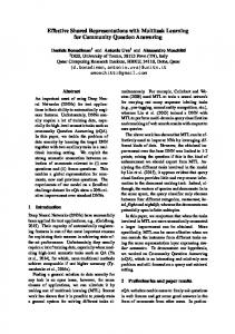
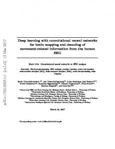
Figure 1: Architecture of the contextual model. (drawn from a finite set of labels) that the viewer intends to watch— hence the problem is formulated as multi-way classification. Prediction is performed at each time step t ∈ [1, n] on each successive voice query qt , exploiting all previous queries in the session [q 1 , . . . , qt −1 ] as context. Given the nature of the domain, this problem seemed like obvious “low hanging fruit” for which a better model would translate into large customer impact. We begin by summarizing our solution, which was previously described in Rao et al. [24] and was recently deployed to production. This model sets the stage for the richer multi-task architecture we present later. The idea of capturing session-level information is operationalized using hierarchical recurrent neural networks. The main intuition is that across queries, the system can accumulate contextual signals to better disambiguate later queries in the same session. In reality, Rao et al. [24] described several model variants, but here we discuss only the complete N-HRNN model, shown in Figure 1. Each query in the session is first run through a shared LSTM (blue rectangles) to produce a sequence of query embedding vectors. They are then fed into another LSTM (rectangles with red dots) to learn the contextual representation of each query in the session, encoded as contextual query vectors c 1 , . . . , c n . These allow the LSTM to find an optimal combination of signals from prior context and the current query. In some cases, the model can learn “relatedness” between successive queries to increase confidence in the desired program. In other cases, the context might actually introduce noise, particularly if the intent is vague. With sufficient data, the model can learn to distinguish between these two cases. The final program prediction is produced by the fully-connected layer, conditioned on the contextual vector of the current query.

4

into production as part of the X1 software package on January 5, 2018. In this section, we describe deployment details and lessons learned from the first month of live traffic. Our experience provides a case study of technology transfer from research into production.

INITIAL MODEL DEPLOYMENT

The model presented above was detailed in Rao et al. [24], where different variants were evaluated retrospectively using query log data. Under these carefully-controlled experimental conditions, the benefits of modeling context were clear. We observed gains over the existing production system, a variety of competitive baselines, and contrastive configurations of the complete model. On a test set of 82K real-world queries, the N-HRNN outperformed a strong neural baseline by 7.5 absolute points in accuracy. Following these promising laboratory experiments, we packaged our N-HRNN into a standalone software module that was deployed

4.1

Implementation Details

To balance efficiency, effectiveness, and coverage, our model was deployed in production as part of a cascade, where the N-HRNN module was run after a number of simpler NLP modules (based on pattern matching and some machine-learned components). A cascade architecture has several advantages: While it would have been possible to run the N-HRNN in parallel with the existing modules, such a setup introduces a new ensemble selection problem that complicates deployment. Since we are introducing completely new technology (this is the first neural network model that has been deployed in production), we adopted a conservative approach to minimize adverse effects. Because the N-HRNN is placed at the end of the cascade, it is given queries that would have otherwise gone unhandled (more details below). Finally, a cascade deployment allows us to control query latencies and to take advantage of richer models only when they are needed (e.g., there is no need to run a deep neural network to respond to the query “CNN”). This is similar in spirit to cascade architectures for ranking [31]. Implemented in Keras with the TensorFlow backend, our model has over 17M parameters, 15M of which come from the embedding matrix. The model is serialized into a 69 MB file and deployed as part of a Docker image. Inference for a single query takes around 70ms on a GPU server (Tesla M60 GPU, Xeon E5-2643 v4 CPU), while latency increases to 750ms on a server with a single Xeon E5-2660 v3 CPU. Since feedforward inference is embarrassingly parallel, we can scale up easily by load balancing across an arbitrary number of servers to obtain the desired throughput. At peak load, we use a small cache to skip model inference for the most frequent N queries, which lowers average latency considerably.

4.2

Query Coverage

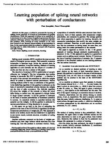
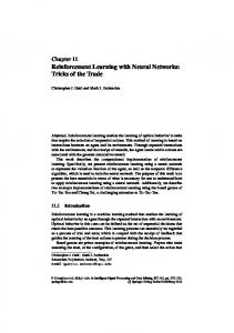
Before we deployed the N-HRNN, the production system was unable to produce any response for 8% of all queries—in this case, the customer sees a special “cannot handle this query” message. Thus, the queries given to our model are the most difficult queries by construction. A manual analysis revealed numerous challenges: speech recognition errors, references to brand new programs, ambiguous intent, or even complete gibberish. By deploying our N-HRNN as the last step of the cascade, we hoped to handle as many of these queries as possible without making too many mistakes. As an additional control mechanism, we implemented a confidence threshold (output of the softmax layer), below which the N-HRNN does not return a response. This threshold, which was hand tuned, allowed us to trade off coverage for precision. After deployment, we monitored logs in the week from January 27 to February 2, 2018: the complete system received 70.1M queries, 5.7M of which (8%) were sent to our N-HRNN, the last step of the cascade. Among these 5.7M queries (for which the viewer would have gotten an error message previously), the model confidence was above the threshold for 4.2M (6%). In other words, the N-HRNN

index=vrex source=VREX_TopN_Commands_Hourly

splunk_server=rexsplk-po-03p.sys.comcast.net| where

    (nlpSource="MOVIE QUOTES" OR nlpSource="dNLP" OR nlpSource="EVENT" OR nlpSource="ENLP" OR nlpSource     ="API.AI" OR nlpSource="FullNLP") | timechart span=1hr count by nlpSource limit=0 from Jan 1 through … ✓ 57,668 events (1/1/18 12:00:00.000 AM to 1/21/18 12:00:00.000 AM)

Sampling 1 : 1,000

Visualization

300

⊖ Reset Zoom

since the alternative was an error message. In the remaining third, where the system provided a non-relevant response, arguably we haven’t made anything worse. Considering these were the most difficult questions to begin with, we were extremely pleased with the coverage and accuracy of our model on live production traffic.

200

API.AI ENLP EVENT FullNLP MOVIE QUOTES dNLP

100

‹

Tue Jan 2 2018

Fri Jan 5

Mon Jan 8

Thu Jan 11

Sun Jan 14

›

4.4

_time

Figure 2: Production traffic deployment. The _time API.AI after ENLP N-HRNN EVENT FullNLP MOVIE QUOTES 2018-01-01 00:00 2 142 module 5 69 fraction of queries served by our (orange) gradually0 2018-01-01 01:00 1 116 2 75 0 replaces queries without any responses (purple). 2018-01-01 02:00 0 144 6 76 0

dNLP

Lessons Learned and Shortcomings

As a first attempt at a challenging problem, our results were very 0 promising and our production deployment surpassed expectations. 0 0 This encouraged us to pursue additional refinements based on the 2018-01-01 03:00 0 127 7 77 0 0 lessons learned. We discuss these points here, which naturally leads 2018-01-01 04:00 0 122 3 76 0 0 to our richer and more ambitious multi-task model in Section 5. received 8% of the total traffic0and responded to 6%;74for the remain2018-01-01 05:00 111 5 0 0 Based on error analysis, we noticed a few systemic problems with 06:00 model chose not to 0 respond, 96 53 0 ing2018-01-01 2%, our and2 the platform resorted0 07:00 1 80 2 38 0 0 the N-HRNN. First, the model takes a classification approach with to2018-01-01 the existing behavior (displaying the error message). 2018-01-01 08:00 0 65 2 15 0 0 a fixed set of programs and cannot generalize to new programs: the Figure 2 shows the breakdown of per-module query coverage. 2018-01-01 09:00 1 36 4 17 0 0 dynamic nature of the entertainment business makes this a critical The main is 32shown at the top (yellow) and0 2018-01-01 10:00pattern-based module 0 0 6 0 11:00 0 28 1 8 other special0 0weakness. On average, 675 new programs are added to our catalog the2018-01-01 N-HRNN is shown in orange at the bottom. A few 2018-01-01 12:00 1 0 every day. For example, many of the non-relevant responses were ized modules (sports, events, 00trivia33 questions, etc.)14 can be seen as00 2018-01-01 13:00 48 1 18 0 for queries about ongoing events, such as the Screen Actors Guild small slivers. After the N-HRNN was unhandled queries0 2018-01-01 14:00 2 78 deployed, 4 29 0 Awards and the Grammys. Queries with an unsupported intent 2018-01-01 15:00 0 75 2 34 0 0 (purple) gradually turned orange. Our N-HRNN quickly became 16:00 1 108 3 40 0 0 type (e.g., “recently purchased” refers to a special menu on the the2018-01-01 second most impactful module in the production system. 2018-01-01 17:00 0 103 1 62 0 0 X1 unknown to our model) also generated non-relevant responses. Based on this, we can conclude that the coverage of the N-HRNN0 2018-01-01 18:00 1 108 5 51 0 2018-01-01 19:00 0 114 53 0 Since our model was only trained on programs, person references module is 74% (4.2M/5.7M). The coverage of6 the entire end-to-end0 were likely to produce non-relevant results as well. Finally, the system increased from 92% to 98% after deployment. In other words, http://splunk.streamsage.com/en-US/app/oiv/search?earliest=1514764800&latest=1516492800&q=search%20index%3Dvrex%20source%3DVREX_TopN_Comman… 1/2 model tends to predict programs for which there are many training our N-HRNN dramatically increased coverage, reducing the number examples—for example, queries mentioning “music” sometimes of unhandled queries by three quarters. yielded a popular channel called “CMT Music”. Generally speaking, there are several fundamental limitations in 4.3 Quality Evaluation our problem formulation: First, our assumption that viewers usually In addition to coverage, we are also interested in accuracy: When the have clear viewing intents is not necessarily correct. Based on our model generates a response, how good is it? And more importantly, log analysis [25], we can identify around one hundred distinct what is the impact on the customer experience? Recall that these intents, most of which are either non-navigational or not viewingqueries were previously not handled and the system responded with related, such as looking for a person or setting reminders. In these an error message. Therefore, any relevant response represents an cases, program prediction makes no sense. Second, a classificationimprovement. Furthermore, it is unclear if a non-relevant response based formulation is unable to handle new programs and also suffers is actually worse than an error message. for tens of thousands of tail programs that have limited training To formally evaluate output quality, we devised a simple threeinstances. In addition, the number of parameters increases linearly grade relevance scale: 1 means the response was completely not with the number of classes in a multi-way classification setting, relevant, 2 means the response was somewhat relevant (i.e., there which has been shown to be neither effective nor efficient when might have been a better response, but the system output was scaling to millions of classes [15]. reasonable), and 3 means the response was completely relevant. Taking a step back, we realized that query understanding actually Every week, our quality assurance team examines a random requires three complementary tasks: sample of queries for which our N-HRNN provided a response: (1) Program prediction (the focus of our previous efforts) to diDuring our evaluation period, this resulted in a dataset of 809 anrectly identify the program or channel referenced in a viewer’s notated queries. The annotator listened to the audio and looked at utterance, out of a catalog of tens of thousands of programs the final output to determine its relevance. Results showed that 29% and hundreds of channels. of responses were graded as completely relevant (e.g., query was (2) Intent classification tries to understand what the viewer “Missoula gumball” and the N-HRNN response was “The Amazing wishes to accomplish. When program prediction (above) idenWorld of Gumball”), while 38% received a grade of 2, somewhat tifies a program or channel with high confidence—it is likely relevant (e.g., “Letterman” led to the movie “Dying to Do Letterthat the viewer wishes to watch the program (or channel). Howman”). Only 33% were considered non-relevant. However, further ever, in some rare cases, the intent is not to watch the show, analysis suggested that these non-relevant responses were usually but to set up the DVR to record the show. This explains the “interpretable” by viewers, e.g., an erroneous partial match (“Ally need for program prediction and intent classification to work Wong” returned “Austin & Ally”). We did not observe many “wildly in conjunction, and both are necessary to properly understand off-base” responses that would perplex the viewer. complex queries. Another prevalent intent is Browse, where In summary, for two thirds of queries that the N-HRNN prothe viewer is looking for something to watch, but does not vided a response (4.2M queries), the customer experience improved,

27H(5 (11.6%) 81.12W1 (3.9%) 5(C25D (1.5%) (17I7Y (1.9%)

CHA11(L (29.7%)

%52W6( (6.5%)

AM%IG8286 (9.1%) M29I( (8.8%) (9(17 (8.8%) 6(5I(6 (18.3%)

Figure 3: Intent distribution based on log analysis.

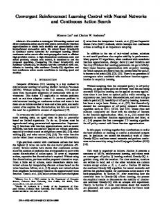
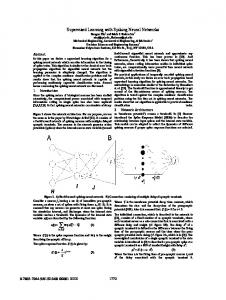
have anything specific in mind. In total, our system recognizes roughly one hundred intents: these range from toggling closed captioning to issuing play/pause/fast forward commands to checking the weather and more. (3) Query tagging works in conjunction with intent classification to provide a fine-grained analysis of queries. Here, the problem is formulated as a sequence labeling task, where we assign a tag to each token. The tag set contains around a dozen domainspecific tags, including “person” (e.g., allowing us to identify names of actors), “categories” (e.g., shows vs. movies), “genre” (e.g., action vs. drama vs. comedy), and a few others. As an example, the intent distribution over a dataset comprising 81M real-world queries is shown in Figure 3 (see Rao et al. [25] for more details). More than half of all traffic is about viewing a specific show: either a channel, a program, or an event. The Browse intent, where viewers do not have a specific program in mind, represents around 6.5% of queries. Examples are “show me free kids movies” or “HD movies with Julia Roberts”. In these cases, the viewer has some idea of the desired program but is expecting suggestions from the system. Beyond View and Browse, our intent taxonomy includes other less frequent categories, such as Entity (1.9%), Record (1.5%), and a few dozen intents that are grouped in Other (11.6%). Although the majority of traffic is about viewing specific programs, handling the “long tail” of intents is critical for improving the overall customer experience. To support such a wide range of capabilities in production, we present a multi-task architecture that jointly learns the above three related tasks. At inference time, models for these three tasks can be deployed to resolve ambiguity and reinforce confidence on clear intents, or they can be used as increasingly-broad backoff mechanisms to cope with queries that have vague intents. For example, if we identify a clear viewing intent and also a specific program, there is a high degree of confidence that the joint prediction is correct. On the other hand, if the system identifies a Browse intent, query tagging results can be used to guide a search-based strategy to narrow down program choices (see example in the introduction). These three tasks provide different perspectives to understand a query, and are both necessary and complimentary in a comprehensive voice search system. We devote the rest of the paper to articulating this much richer architecture.

5

MULTI-TASK LEARNING ARCHITECTURE

In this section, we present our multi-task learning architecture with detailed explanations about model design for program prediction, intent classification, and query tagging. These three tasks share the contextual component of the N-HRNN as a base module to convert an input voice session to a semantic embedding, on top of which task-specific models are separately built. Given a voice query session [q 1 , . . . , qn ], we jointly make three types of predictions: (1) the program that the viewer intends to watch for each query, (2) an intent type for each query, and (3) a tag sequence for each query. The three tasks are performed on each successive new voice query qt (t ∈ [1, n]), exploiting all previous queries in the session [q 1 , . . . , qt −1 ] as context. At each time step t, the model makes all predictions concurrently. To exploit the benefits of jointly performing these three complimentary tasks, we adopt a multi-task learning strategy to train the entire network in an end-to-end manner. The overall model architecture is shown in Figure 4 and consists of three distinct components: (1) Query embedding component, shown in the bottom lookup layer and the blue BiLSTM: the lookup layer converts a raw query string to a sequence of vectors (through word2vec [19]) and the BiLSTM learns a semantic embedding for the query. More formally, given a query qt represented as a sequence of words {wt }, the output is a sequence of hidden vectors {hbi t } learned from the BiLSTM. The last hidden vector is used as the query embedding vt , which is passed to the contextual component. The sequence of hidden vectors {hbi t } serves as input to the tagging model to generate a word-level tag sequence. (2) Contextual component, shown as the red-dotted rectangles, is the same as the corresponding LSTM in Section 3. It takes all the preceding query embeddings {v 1 , ..., vt } as context to produce a contextual vector c t that captures both semantic and contextual features. The contextual vectors {c t } are then fed into the intent classification and program prediction components. (3) Task-specific components for query tagging (the yellow rectangle), intent classification (the pink rectangle), and program prediction (the red rectangle). At the top, we weight the losses from the three tasks and sum them together for unified multi-task learning. Details of the three task components are provided in Sections 5.1– 5.3, and multi-task optimization in Section 5.4.

5.1

Program Prediction

Our first task-specific component is responsible for program prediction, which models the probability P (p|c t ) of generating program p given the contextual vector c t for an ongoing session {q 1 , ..., qt }. Unlike the N-HRNN model that treats program prediction as multiway classification (and thus is unable to handle rarely-watched tail programs and newly-added programs), we model the task as a ranking problem (i.e., modeling the relevance between a query and a program). Our model introduces a novel triplet ranking approach that can directly exploit interactions between training (query, positive program, negative program) triples and can take advantage of program embeddings to integrate different sources of evidence (e.g., program title, viewers’ search and viewing histories) in a flexible manner. The learned program embeddings are paired with the

Sum(loss)

⊕ Tagging c1 q1

q2

Program Prediction q3 q2 q1

Intent Classification c2

q3

c3 b

HierLSTM

⊗

b

b

b

b

b

b

b

b

b

b

b

b

b

b

b

b

b

b

b

b b

bc b

b

b

b

b

b

b

b

b

b

b

Program Embedding

BiLSTM

Layer

Lookup Layer q1 :“Go HBO Channel ”

Lookup Layer q2 :“Game of Throw”

Lookup Layer q3 :“Game of Throne”

b

p

+

− p− 1 p2

b

b

p− n

Figure 4: Our multi-task learning architecture, which contains three distinct components: (1) a query embedding component at the bottom (blue rectangles) that converts a query string to a learned representation, (2) a contextual component (red dotted rectangles) that models the context between queries in a session, and (3) task-specific components designed for three tasks: program prediction (in red), intent classification (in pink), and query tagging (in yellow). query embeddings in a triplet loss to identify the most relevant program in a contrastive manner. In our model, a channel (e.g., “HBO”) is treated exactly like a program. Let Φ denote the set of all programs in the training dataset. We reformulate maximizing the classification probability P (p|c t ) as a ranking objective: P (rel | c t , p + ) > P (rel | c t , p − ), ∀p + , p − ∈ Φ That is, we wish to assign a higher relevance score to positive programs from the training data than any negative program. We propose three ways to learn a program embedding: (1) Search-based program embeddings. We can define programs purely based on how viewers search for them. In this representation, the program embedding layer is a simple lookup layer that maps a program id (scalar) to a learned embedding vector, which is randomly initialized and updated during training. Our assumption is that given enough data, the embeddings will converge to a meaningful representation, reflecting how viewers search for programs. This is similar to how word2vec [19] is trained from neighboring word associations; in our case, we use search-based associations instead. Like word2vec, such representations can overcome lexical mismatches. For example, viewers may search for a channel by its number (i.e., “210” → “HBO”), where there is no lexical overlap; this representation can learn such correspondences from log data. However, the drawback of this search-based representation is its dependence on observations; it is unable to handle cases where the viewer refers to an unseen program. From this representation, the relevance score between an ongoing session {q 1 , ..., qt } and a program can be measured by the cosine similarity between the program embedding p and the contextual vector c t : P (rel | p, q 1 , ..., qt ) = P (rel | p, c t ) = cosine(p, c t )

(2) Title-based program embeddings. As an alternative, we can model query–program similarity lexically. To accomplish this, we copy the query embedding component as our program embedding layer and apply it to the program title, from which we obtain another sequence of BiLSTM vectors representing the program. Let the query representation be {hbi q } and the program representation be {hbi p }. We adopt an interaction-based method (similar to [26]) to model the similarity between each word pair in (query, program): bi sim(i, j) = cosine(hbi q [i], hp [j])

From this we obtain a similarity matrix where each entry (i, j) denotes the cosine similarity between query word i and program title word j. We apply max pooling along the rows, which returns a query-sized feature vector. Each feature i denotes the highest similarity between any program title word and query word i. To capture the relative importance of different query words, we weight this feature vector (element-wise) by inverse document frequency (IDF). Similarly, we repeat the same operation along the columns to obtain a program-sized feature vector, where each element j denotes the highest similarity between any query word and program title word j (also IDF-weighted). These two feature vectors are concatenated and passed to a linear layer, which computes a relevance score for the query–program pair. (3) Combination-based program embeddings. To capture the best of both representations, we stack another linear layer on top to combine the search-based and title-based relevance scores. This can be considered a linear learning-to-rank approach with only two feature inputs. At this point, we have introduced three approaches for computing the relevance of a program with respect to the current query in the session. Given such a relevance scoring function P (rel), we explore

the interactions between positive and negative programs through a softmax function: exp(P (rel | p + , q 1 , ..., qt )) ′ p ′ ∈C exp(P (rel | p , q 1 , ..., q t ))

o[p + ] = P (p + |q 1 , ..., qt ) = P

where p + is the positively labeled program for session i, o[p + ] denotes the probability of predicting p + , and C denotes the set of candidate programs to be ranked. Ideally, C should be equal to the program set Φ; in practice, we approximate this through negative sampling, by selecting k (e.g., k = 10) programs from the top ranked results of query qt using a standard retrieval algorithm (i.e., BM25). Our goal is to maximize the likelihood of generating positive programs given queries across the dataset, which can be equivalently formulated as minimizing the program loss function: Lp = −

|D | X n X

log oi [p + ] = −

i=1 t =1

|D | X n X

log P (p + |q 1 , ..., qt )

i=1 t =1

where the outer sum iterates over all sessions in the dataset D, and the inner sum iterates over all queries in session i.

5.2

Intent Classification

Similar to program prediction, we also aim to predict the intent type at for query qt given its contextual vector c t . We model this task as a classification problem since the vocabulary of intent types is relatively small and stable. On the top section of Figure 4 (the pink rectangle labeled “Intent Classification”), a fully-connected layer followed by a softmax layer defines the classification function. The fully-connected layer consists of two linear layers with a ReLU element-wise activation layer in between. The contextual vector c t is fed into the fully-connected layer first, followed by L1 normalization via the softmax function, producing normalized output vector o. Each output score o[a j ] denotes the probability of predicting intent type a j as output. The intent classification loss is summed over all queries in the dataset, as follows: Li = −

|D | X n X

log P (at |c t ) = −

i=1 t =1

5.3

|D | X n X

log ot [at ]

i=1 t =1

Query Tagging

Unlike program prediction and intent classification, which are query-level predictions, query tagging is a sequence labeling task. More formally, our query tagging component takes the output vector sequence {hbi t } from the bottom BiLSTM as input and generates a tag sequence {τt }, where each tag label corresponds to a word in the query qt . We use a conditional random field (CRF) [16] as our tagging model (the yellow rectangle labeled “Tagging” in Figure 4) on top of the BiLSTM. In addition to capturing the neighboring word context through the BiLSTM, a CRF can exploit correlations between tag labels in neighborhoods to jointly decode the best label sequence for a given query. We use standard maximum likelihood estimation for training the CRF and the Viterbi algorithm for decoding. We omit the technical description of CRFs for space reasons, but refer readers to Lafferty et al. [16] for details.

5.4

Multi-Task Learning

Since the three tasks have their own optimization objectives, we adopted a multi-task learning strategy to train our entire model end to end, jointly optimizing all three tasks. This is accomplished in two stages: Following a commonly adopted strategy [17, 20], in the first stage, all tasks are jointly trained by summing up their losses based on a mixing ratio. Let wp , w i , and w t be the contribution weight to the combined loss from each task (program prediction, intent classification, and query tagging, respectively). The overall loss is computed as follows: L = w p · Lp + w i · L i + w t · L t where wp , w i , and w t sum to 1.0. In the second stage, we freeze the underlying shared layers (the bottom BiLSTM and hierarchical LSTM layer) and fine-tune the top task-specific layers (including the program embedding layer) with task-specific losses.

6 EXPERIMENTAL SETUP 6.1 Data Collection To build a dataset for supervised learning, we need the following for each session: the program title (one per session), the intent type (one per query), and query tags (one for each query word). We use a combination of user logs and human annotations to obtain such data. The program title is extracted entirely from logs, in a manner analogous to harvesting clickthroughs in the web domain: If the viewer began watching program p after the final query in a session and continued watching it for at least 150 seconds, we label the session with p (this duration parameter was explored in Rao et al. [24]). For the intent type and the query tags, we used a semi-supervised approach to collect ground truth data. Initially, hand-crafted patterns were manually designed by our annotation team, which were then applied to parse queries into a logical form, from which we extracted the intent type and query tags. New patterns were gradually added over time to increase coverage. This bootstrapping process can be thought of as a simple yet practical human annotation strategy when exhaustive hand-labeling is infeasible in a large-scale setting. Using this process, we extracted a total of 8.8M training instances (labeled sessions) from 81.4M queries received during the week of February 22 to 28, 2017, from which we randomly sampled a subset and split into training, validation, and test sets. The set of intent types and query tag types were extracted based on a particular set of hand-crafted patterns at a particular point in time. Basic statistics are summarized in Table 1. All three sets are sufficiently large to realistically capture the diversity of viewer queries. The percentage of single-query vs. multi-query sessions is about 80:20 for all three sets. The program set contains 26247 distinct programs and 244 channels. About 10% of the queries in the validation and test sets have program labels that are not seen in the training set. There are 109 intents and 11 tag types in total.

6.2

Model Training

We used 300-dimensional word2vec [19] embeddings to encode each word, trained on the Google News dataset and freely available. The word vocabulary of the training set is 29.3K and 4282 lack word2vec vectors; these were randomly initialized with values uniformly

Dataset Train Validation Test

Sessions Queries Avg. Sess. Len Avg. Q. Len 870,941 1,186,937 1.36 2.24 623,142 823,565 1.32 2.23 622,959 825,639 1.33 2.23 Table 1: Dataset statistics.

sampled from [−0.05, 0.05]. Words in the validation and test sets unseen during training were treated as out of vocabulary. During training, we used stochastic gradient descent together with the Adam optimizer to iteratively update model parameters. The learning rate was initially set to 10−3 and then decreased by a factor of three when the validation set loss stopped decreasing for three epochs. The LSTM output size and the size of the linear layers were set to 150. The batch size was set to 256. For each task, the model parameters that obtained the lowest task-specific loss on the validation set was used at evaluation time. During evaluation, as input candidates for our model to rerank, we used the top 20 programs retrieved by BM25 on character-level 3-grams from the program titles (see baseline condition below). We also add all channels into our candidates pool when the detected viewer intent is to view a channel. This helps cases where the query and program share no lexical overlap (i.e., the query is a channel number and the “program” is the channel name). Our models were implemented using Keras, running on a server with 8 GPUs (GeForce GTX TITAN X) and 256GB RAM. In order to demonstrate the effectiveness of multi-task learning, we compared two different approaches for training our models: Single-Task Learning (STL). Although our architecture is designed for multi-task learning, it can still be trained for a single task. In this mode, the training process only optimizes the intended task loss (e.g., intent classification), while ignoring losses from the other two tasks (by assigning zero to their mixing weights). Typically, the training process converges in five epochs and each epoch takes about 1.5 hours. Multi-Task Learning (MTL). For multi-task learning, we used the two stage approach described in Section 5.4. For tuning the weights of the individual task-specific loss, we performed cross-validation on the validation set to select the best mixing ratio that minimizes the weighted sum of the three task-specific losses. In practice, we found a mixing ratio of (0.55, 0.05, 0.4) for program prediction, intent classification, and query tagging, respectively, worked well for the search-based representation, and (0.1, 0.2, 0.7) worked well for the title-based and combination-based representations. Compared to STL, the MTL training process takes much longer, typically 15 epochs per stage.

6.3

Metrics and Baselines

Intent classification and query tagging were evaluated in terms of accuracy. For program prediction, we used three metrics (averaged over all queries): precision at one (P@1), precision at five (P@5), and Mean Reciprocal Rank (MRR). Use of these metrics was motivated by the precision-oriented nature of television navigation, as limited input options require our system to satisfy viewers’ queries as quickly as possible. A number of baselines are described below;

note that some baselines are designed for a particular task, while others can be extended to all three tasks. BM25: We built a 3-gram (character-level) inverted index of the program set Φ. During retrieval, the match score is computed on 3-gram overlaps between the query and program titles using Okapi BM25 weighting (k 1 = 1.2, b = 0.75). SVMrank [14]: We reused the learning-to-rank baseline in our previous work [24], which includes exact and soft-match features (BM25 and embedding-based) as well as popularity priors. DSSM [12]: This neural ranking model, originally designed for web search, uses word hashing to model interactions between queries and programs at the level of character 3-grams. This provides an appropriate baseline since it can handle noisy ASR output, unlike neural ranking models based primarily on word matching [8, 21]. DSSM+S: Using the same model as above, we concatenate queries in one session with a special boundary token between neighboring queries. Our goal here is to examine whether simple query concatenation is sufficient to capture context signals in a session. Stanford CRF Tagger2 [7]: As a standard baseline for sequence labeling, we trained a linear CRF that combines standard local and global features, including features based on n-grams, context windows, etc. N-HRNN with LSTM/BiLSTM [24]: Our original model, as described in Section 3, can be extended to intent classification and query tagging by adding separate fully-connected layers for each task. We also tried both a unidirectional and a bidirectional bottom LSTM layer to examine the effects of bidirectional query modeling.

7

RESULTS

Results for all three tasks are shown in Table 2. Each row represents an experimental setting (numbered for convenience). The second column specifies the model, and the remaining columns show results for program prediction, intent classification, and query tagging, respectively. MTLA refers to our multi-task learning architecture, described in Section 5, trained either using the single-task learning or multi-task learning conditions outlined in Section 6.2. Results are shown in the two subtables titled “Single-Task Learning” and “Multi-Task Learning”, respectively.

7.1

Program Prediction

First, we can see that BM25 achieves reasonably-high accuracies (P@1 of 0.674) on the test set. The SVMrank predictor achieves slightly better accuracy than BM25 by taking advantage of multiple hand-crafted features in a supervised setting. Taking a closer look at the learned model weights, we find that these additional features are largely dominated by the BM25 feature and provide only modest benefit to the overall model. DSSM significantly outperforms SVMrank as well as BM25, whereas DSSM+S performs slightly worse than DSSM, suggesting that simple query concatenation is not able to capture context signals in a session. As expected, the N-HRNN is able to outperform the other baselines by quite a bit. We identified two main reasons: (1) There are about 3% of queries (about 10% of all channel-intent queries) in which the viewer searched for a particular channel by memorizing 2 https://nlp.stanford.edu/software/CRF-NER.shtml

Program P@1 P@5 MRR BM25 0.674 0.750 0.711 SVMrank 0.682 0.758 0.718 DSSM 0.703 0.765 0.732 DSSM+S 0.699 0.758 0.728 Stanford CRF Tagger N-HRNN LSTM 0.724 0.783 0.755 N-HRNN BiLSTM 0.725 0.786 0.753 Single-Task Learning MTLA (search-based) 0.715 0.770 0.744 MTLA (title-based) 0.720 0.796 0.754 MTLA (comb-based) 0.738 0.802 0.768 Multi-Task Learning MTLA (search-based) 0.721 0.780 0.758 MTLA (title-based) 0.728 0.803 0.762 MTLA (comb-based) 0.757 0.812 0.792

ID Model 1 2 3 4 5 6 7 8 9 10 11 12 13

Intent Tagging Accuracy 0.821 0.915 0.884 0.916 0.939

0.917

0.944

0.923 0.924 0.925

0.946 0.945 0.945

Table 2: Model effectiveness for different experimental settings. MTLA refers to our multi-task learning architecture, trained either using the single-task learning or multi-task learning conditions. Columns show results for program prediction, intent classification, and query tagging.

its channel number; (2) Major ASR errors sometimes result in very little lexical overlap between the query and the intended program title (e.g., “Dr. Seuss’s The Lorax” is transcribed as “The Laura”). In both cases, the query and the program title (or channel) have minimal 3-grams overlap (or none), so approaches based on lexical matching (e.g., DSSM) cannot predict the correct program. We further examine the session context by decomposing the dataset into single-query and multi-query sessions. Comparing DSSM and N-HRNN, the accuracy gap is much larger on multi-query sessions (P@1 of 0.546 vs. 0.483) than on single-query sessions (P@1 of 0.770 vs. 0.757), thus affirming the value of modeling session context. Single-query sessions obtain much higher accuracies overall since they are by construction “easy queries” in which viewers reach their intended program in a single query. These findings are consistent with Rao et al. [24]. Finally, we see that bidirectional modeling (BiLSTM) provides little benefit for program prediction. Turning our attention to the “Single-Task Learning” subtable (rows 8–10), we observe that the search-based program representation performs worse than the N-HRNN model. Considering that these two models share the same underlying query embedding and contextual component, the difference comes from the problem formulation (classification vs. ranking) and how we train the model. In the search-based model, we selected k negative programs for each query–program sample during training. This can be less effective than a classification formulation since the classification loss forces the N-HRNN to select the positive program against all negative programs, thus giving it stronger discriminative power. However, this does not mean that a classification approach is better, as we discussed in Section 4.4. The ranking formulation works well with the combination-based representation (row 10), which significantly outperforms N-HRNN at p < 0.05 using Fisher’s two-sided, paired randomization test [30]. Incorporating signals based on program

Intent Channel Movie Series Event Browse Channel 97.9% 0.4% 0.5% 0.0% 0.2% Movie 0.4% 89.7% 2.4% 0.1% 3.3% Series 0.2% 0.8% 96.2% 0.0% 1.3% Event 0.4% 3.7% 1.6% 87.3% 0.0% Browse 0.1% 1.9% 1.8% 0.0% 94.1% Table 3: Confusion matrix for the top five intent types, where the rows indicate the actual labels and the columns the predicted labels.

titles helps the combination-based approach answer queries about programs not observed during training, which cannot be answered using a classification approach. Subtable “Multi-Task Learning” (rows 11–13) confirms the benefits of multi-task learning. Regardless of program representation, program prediction is consistently and significantly (p < 0.05) better than training in isolation. As expected, the improvements from multi-task learning come from partial task overlap with intent classification and query tagging. High confidence in a predicted intent is able to help the program prediction component discard candidate outputs that conflict. For example, the query “Disney channel shows” is predicted as having intent Browse, and so the predicted program is correctly set to NA (no answer).

7.2

Intent Classification

As shown in the “Intent” column in Table 2, the N-HRNN variants form strong baselines, suggesting that intent classification is an easier problem due to the limited size of the intent set. Bidirectional modeling doesn’t improve the accuracy here. Since the approaches in subtable “Single-Task Learning” are essentially the same model as the N-HRNN BiLSTM (with respect to intent classification), the accuracy differences are negligible. However, by jointly learning all three tasks, we see consistent improvements. Our best method (combination-based) achieves an accuracy of 0.925, which we consider quite impressive given the diversity of real voice queries. For further insights, we show the confusion matrix of our best method (combination-based) for the most frequent five intent types in Table 3 (where the rows indicate the actual labels and the columns the predicted labels). The Channel intent has the highest accuracy, while the Event intent has the lowest accuracy. This matches our intuition that channel tuning is an easier task while the Event intent is harder to identify given its somewhat vague definition. We also see that the model is often confused between the remaining three intent types: Movie, Series, and Browse. Again, this is likely due to blurred lines between these intent types. For example, the query “life of pets” can be interpreted either as an intent to watch the movie with that title, the television series, or to Browse the catalog for documentaries about pets.

7.3

Query Tagging

In the final “Tagging” column in Table 2, we see that the CRF tagger achieves the lowest accuracy of 0.821 among all baselines: the N-HRNN LSTM outperforms the CRF-only approach by more than six absolute points. Unlike the other two tasks, bidirectional modeling is crucial for the tagging problem because the tag of a

1

Stanford CRF Tagger Single LSTM Single BiLSTM Multi-Task(comb)

0.8

0.6

0.4

0.2

0

Context

Channel

Title

Genre

Person

Figure 5: Tagging accuracy of all methods for five tags. particular word is dependent on both the previous and next words. By introducing a CRF on top of the BiLSTM in our multi-task model (with “Single-Task Learning”), we are able to significantly beat the N-HRNN BiLSTM and CRF baselines (p < 0.05). Finally, multi-task learning provides an additional small boost to tagging accuracy. Not all tags are created equal, which is why we examined the accuracies of various methods for five representative tags, shown in Figure 5. For the most common three tags (context, channel, and title) that make up 95% of tokens, our multi-task learning approach consistently performs the best while the CRF performs poorly. However, the CRF performs well on the least frequent tags (genre and person). This is likely due to insufficient training data for these tags (each appears in less than 1.5% of tokens). The LSTM-based approaches have a much larger parameter space, making them more data hungry. Overall, our best multi-task approach achieves a tagging accuracy of nearly 95%. Once again, we believe that these results are quite impressive given the diversity of real-world queries.

8

NEXT STEPS AND CONCLUSIONS

Our vision is that future entertainment systems should behave like speech-enabled intelligent agents. In this paper, we described our current progress toward this goal. Initial efforts focused on picking the “low hanging fruit” of navigational voice queries. Today, our N-HRNN runs in production as part of the Comcast X1 platform, and the model has improved the customer experience for millions of queries each day. To tackle the limitations of our initial solution, we designed a novel neural architecture to jointly accomplish three related tasks: program prediction, intent classification, and query tagging. This paper articulates how the three tasks complement each other to understand a wide range of intents. We demonstrate how joint learning improves the effectiveness of each task individually, yielding significant gains over strong baselines. More importantly, our multi-task framework provides an opportunity to build a complete end-to-end system for understanding voice queries. This new model is now being prepared for deployment and will soon be serving millions of Comcast customers, providing natural voice-based interactions for the entertainment domain.

REFERENCES [1] R. Caruana. 1997. Multitask Learning. Machine Learning (1997), 41–75. [2] O. Chapelle and Y. Zhang. 2009. A Dynamic Bayesian Network Click Model for Web Search Ranking. WWW. 1–10. [3] C. Chelba and J. Schalkwyk. 2013. Empirical Exploration of Language Modeling for the google.com Query Stream as Applied to Mobile Voice Search. Mobile Speech and Advanced Natural Language Solutions. [4] R. Collobert and J. Weston. 2008. A Unified Architecture for Natural Language Processing: Deep Neural Networks with Multitask Learning. ICML. 160–167. [5] M. Dundar, Q. Kou, B. Zhang, Y. He, and B. Rajwa. 2015. Simplicity of K-means Versus Deepness of Deep Learning: A Case of Unsupervised Feature Learning with Limited Data. ICMLA. 883–888. [6] J. Feng and S. Bangalore. 2009. Effects of Word Confusion Networks on Voice Search. EACL. 238–245. [7] J. Finkel, T. Grenager, and C. Manning. 2005. Incorporating Non-local Information into Information Extraction Systems by Gibbs Sampling. ACL. 363–370. [8] J. Guo, Y. Fan, Q. Ai, and B. Croft. 2016. A Deep Relevance Matching Model for Ad-hoc Retrieval. CIKM. 55–64. [9] I. Guy. 2016. Searching by Talking: Analysis of Voice Queries on Mobile Web Search. SIGIR. 35–44. [10] A. Hassan, R. Kulkarni, U. Ozertem, and R. Jones. 2015. Characterizing and Predicting Voice Query Reformulation. CIKM. 543–552. [11] H. He, J. Wieting, K. Gimpel, J. Rao, and J. Lin. 2016. UMD-TTIC-UW at SemEval2016 Task 1: Attention-Based Multi-Perspective Convolutional Neural Networks for Textual Similarity Measurement. SemEval. 1103–1108. [12] P. Huang, X. He, J. Gao, L. Deng, A. Acero, and L. Heck. 2013. Learning Deep Structured Semantic Models for Web Search using Clickthrough Data. CIKM. 2333–2338. [13] J. Jiang, W. Jeng, and D. He. 2013. How Do Users Respond to Voice Input Errors? Lexical and Phonetic Query Reformulation in Voice Search. SIGIR. 143–152. [14] T. Joachims. 2006. Training Linear SVMs in Linear Time. SIGKDD. 217–226. [15] A. Joulin, E. Grave, P. Bojanowski, and T. Mikolov. 2016. Bag of Tricks for Efficient Text Classification. arXiv:1607.01759. [16] J. Lafferty, A. McCallum, and F. Pereira. 2001. Conditional Random Fields: Probabilistic Models for Segmenting and Labeling Sequence Data. ICML. 282–289. [17] P. Liu, X. Qiu, and X. Huang. 2017. Adversarial Multi-task Learning for Text Classification. arXiv:1704.05742. [18] M.-T. Luong, Q. Le, I. Sutskever, O. Vinyals, and L. Kaiser. 2015. Multi-task Sequence to Sequence Learning. arXiv:1511.06114. [19] T. Mikolov, W. Yih, and G. Zweig. 2013. Linguistic Regularities in Continuous Space Word Representations. HLT/NAACL. 746–751. [20] R. Pasunuru and M. Bansal. 2017. Multi-Task Video Captioning with Video and Entailment Generation. arXiv:1704.07489. [21] J. Rao, H. He, and J. Lin. 2016. Noise-Contrastive Estimation for Answer Selection with Deep Neural Networks. CIKM. 1913–1916. [22] J. Rao, H. He, and J. Lin. 2017. Experiments with Convolutional Neural Network Models for Answer Selection. SIGIR. 1217–1220. [23] J. Rao, H. He, H. Zhang, F. Ture, R. Sequiera, S. Mohammed, and J. Lin. 2017. Integrating Lexical and Temporal Signals in Neural Ranking Models for Social Media Search. Neu-IR. [24] J. Rao, F. Ture, H. He, O. Jojic, and J. Lin. 2017. Talking to Your TV: Context-Aware Voice Search with Hierarchical Recurrent Neural Networks. CIKM. 557–566. [25] J. Rao, F. Ture, and J. Lin. 2018. What Do Users Say to Their TVs? An Analysis of Voice Queries to an Entertainment System. SIGIR. [26] J. Rao, W. Yang, Y. Zhang, F. Ture, and J. Lin. 2018. Multi-Perspective Relevance Matching with Hierarchical ConvNets for Social Media Search. arXiv:1805.08159. [27] R. Sequiera, G. Baruah, Z. Tu, S. Mohammed, J. Rao, H. Zhang, and J. Lin. 2017. Exploring the Effectiveness of Convolutional Neural Networks for Answer Selection in End-to-End Question Answering. Neu-IR. [28] J. Shan, G. Wu, Z. Hu, X. Tang, M. Jansche, and P. Moreno. 2010. Search by Voice in Mandarin Chinese. INTERSPEECH. 354–357. [29] M. Shokouhi, U. Ozertem, and N. Craswell. 2016. Did You Say U2 or YouTube? Inferring Implicit Transcripts from Voice Search Logs. WWW. 1215–1224. [30] M. Smucker, J. Allan, and B. Carterette. 2007. A Comparison of Statistical Significance Tests for Information Retrieval Evaluation. CIKM. 623–632. [31] L. Wang, J. Lin, and D. Metzler. 2011. A Cascade Ranking Model for Efficient Ranked Retrieval. SIGIR. 105–114. [32] Y. Wang, D. Yu, Y. Ju, and A. Acero. 2008. An Introduction to Voice Search. IEEE Signal Processing Magazine, 29–38. [33] R. Yu, A. Li, V. Morariu, and L. Davis. 2017. Visual Relationship Detection with Internal and External Linguistic Knowledge Distillation. ICCV. 1974–1982. [34] R. Yu, H. Wang, and L. Davis. 2018. ReMotENet: Efficient Relevant Motion Event Detection for Large-Scale Home Surveillance Videos. WACV. [35] B. Zhang and M. Al Hasan. 2017. Name Disambiguation in Anonymized Graphs using Network Embedding. CIKM. 1239–1248. [36] Y. Zhang and Q. Yang. 2017. A Survey on Multi-Task Learning. arXiv:1707.08114.