IEEE TRANSACTIONS ON ANTENNAS AND PROPAGATION, VOL. 54, NO. 2, FEBRUARY 2006
715
Multigrid ADI Method for Two-Dimensional Electromagnetic Simulations Shumin Wang and Ji Chen
Abstract—We propose a multigrid alternating-direction implicit (ADI) method for solving two-dimensional Maxwell’s equations. This method is based on interpreting the ADI method as an iterative solver for the Crank–Nicolson (CN) scheme. By introducing a special procedure to solve the residual equation within the ADI framework, multigrid methods are incorporated into the iterative ADI method. The accuracy and efficiency of the proposed method are further demonstrated by numerical examples. Index Terms—Alternating-direction implicit (ADI) method, iterative methods, multigrid methods.
I. INTRODUCTION
T
HE alternating-direction implicit (ADI) method is a promising unconditionally stable finite-difference timedomain (FDTD) scheme for spatially oversampled problems [1]–[8]. Comparing with other unconditionally stable schemes that typically require to solve general sparse linear systems, the ADI method only involves tri-diagonal matrices that can be solved very efficiently by the Gaussian elimination [13]. Although its time-step size is no longer limited by the Courant– Friedrichs–Lewy (CFL) condition [11], [12], the increasing numerical dispersion error and the splitting error are major drawbacks when the time-step size becomes large. It has been reported that the numerical dispersion error of the ADI method is larger than that of Yee’s scheme [3], [4]. Dispersion error is common in finite methods and primarily affects simulations of electrically large or highly resonant structures. The unique error associated with the ADI method is the splitting error [11], which is proportional to the square of the time-step size and the spatial variation of field [5], [6]. This error has a detrimental effect because large time-step size is the main benefit of using the ADI method and often times, field variation is of interest by itself. Since the splitting error exists at every grid location, it affects not only those electrically large ones, but all simulations. In practice, splitting error is dominant even with modestly large CFL numbers in ADI simulations [7]. To reduce the splitting error, the iterative ADI method has been proposed in [6] where the traditional ADI method is considered as a special case of the general iterative one. In the iterative scheme, the splitting error can be significantly reduced by
Manuscript received November 8, 2004; revised August 6, 2005. This work was supported in part by the NSF under Grant BES-0332957 and in part by the Texas Higher Education Coordinating Board under G rant 003652-0195-2001. S. Wang is with the National Institute of Health, Bethesda, MD 20892, USA (e-mail:
[email protected]). J. Chen is with Department of Electrical and Computer Engineering, University of Houston, Houston, TX 77204 USA. Digital Object Identifier 10.1109/TAP.2005.863093
increasing the number of iterations or using better initial guess. A more efficient approach, the pre-iterative ADI method, was further proposed in [8]. The pre-iterative ADI method utilizes the fact that the splitting error is local in nature. It provides better initial guess by applying additional number of iterations in regions where large splitting error is expected. The iterative ADI method is essentially an iterative matrix solver for the Crank–Nicolson (CN) scheme [6]. For iterative matrix solvers, multigrid is an effective way to improve the conarithmetic operations and vergence rate [15]. Because storage units are required asymptotically to solve unknowns, multigrid method is optimal. In the past, multigrid methods have been applied to various methods in computational electromagnetics, such as the method of moments [16], transmission line matrix method [17], and the finite-element method [18], [19]. In this paper, we incorporate multigrid into the iterative ADI method by using TE waves in lossy medium to demonstrate the main procedure. Since the framework of the multigrid ADI method does not change in the TM case, we only discuss the TM implementation briefly. We also need to point out that in some literatures on the FDTD method, the term “multigrid” also refers to sub-gridding techniques [14]. Here, this term uniquely refers to the aforementioned matrix solving technique. The rest is organized as follows. For ease of understanding and completeness of formulation, we shall first review the iterative ADI method and multigrid methods in Sections II and III respectively. The incorporation of multigrid methods into the iterative ADI method is detailed in Section IV. In Section V, numerical examples demonstrate the validity and efficiency of the proposed method. Finally, conclusions are drawn in Section VI. II. THE ITERATIVE ADI METHOD waves in 2-D lossy medium, we use the following For linear operators to cast Maxwell’s equations [8]: (1) where
and
Note that in the above equation, has been normalized by . By applying the CN scheme at time step [11], we have
0018-926X/$20.00 © 2006 IEEE
(2)
716
IEEE TRANSACTIONS ON ANTENNAS AND PROPAGATION, VOL. 54, NO. 2, FEBRUARY 2006
This is equivalent to the following:
III. MULTIGRID METHODS Multigrid methods utilize the smoothing property of many relaxation solvers. For a linear system of equations (10)
(3) which naturally defines a relaxation method for iteratively solving the CN scheme [20], i.e.
(4) iterative solution. This iterative where subscript denotes the solving procedure can be implemented in the ADI framework in two steps, i.e.
(5)
the solution error of a relaxation method can be defined by (11) the solution after where represents the exact solution and iterations. Relaxation solvers with smoothing property can effectively eliminate high frequency (oscillatory) part of the solution error, but are less effective on the low frequency (smooth) part. By noticing that smooth components on fine meshes become more oscillatory on coarse meshes [15], it is reasonable to transfer the problem to coarse meshes in a way that the same relaxation solver can effectively eliminate the oscillatory part of the solution error on coarse meshes, which are originally smooth on fine meshes. This is the main idea behind coarse grid correction in multigrid methods. Coarse grid correction is performed on the residual equation. If we denote residual from (10) and (11) as
in the first step and
(12) the residual equation can be derived as (6)
denotes an intermediate solution. in the second step, where If we set the initial guess of , i.e. , to be the previous time-step value , we obtain from (5) and (6) (7) and (8) which recover the traditional ADI scheme [5]. Multiplying with (7) and with (8) yields the equation that the traditional ADI method actually solves, i.e.,
(9) which introduces a splitting error term
to the exact solution of (3). The splitting error is essentially due to the fact that the traditional ADI method only applies the iterative ADI method with one iteration and a special initial guess. By fully exercising the iterative solving procedure, the iterative ADI method provides a systematic way to obtain more accurate results. This has been demonstrated in [6], [8].
(13) To start with, an iterative solver is first applied on a fine mesh to obtain solution after iterations. Then the residual on the fine mesh, , is calculated according to (12) and mapped by restriction operator . The mapped to a coarse mesh is substituted into (13) and the solution error on residual is obtained by the same relaxation solver the coarse mesh on . The solution error is finally mapped back to by to obtain the solution error on the interpolation operator . A common requirement for the pair of intergrid fine mesh transfer operators is (14) where is a constant and “ ” denotes transpose [15]. According is a better solution now. Because excites to (11), oscillatory modes on from smooth modes on [15], the relaxation method needs to be applied again. The above procedure fulfills the simplest -cycle and is illustrated in Fig. 1. -cycle can be repeated until a solution with desired accuracy is obtained. Coarse grid correction can be used again to find a better soon . In this scenario, an even coarser mesh lution of , restriction operator , and interpolation operator are constructed. This procedure can be applied recursively to higher levels with more complicated -cycle or other forms of coarse grid correction, e.g., W-cycle [15]. As coarse grid correction focuses on improving the convergence rate of relaxation solvers, multigrid methods use nested iteration to provide better initial guess [15]. Nested iteration is based on the fact that coarse meshes can be used to compute an improved initial guess for relaxations on fine meshes. In this
WANG AND CHEN: MULTIGRID ADI METHOD FOR 2-D ELECTROMAGNETIC SIMULATIONS
717
by restriction operator and restricted to the coarse mesh . We define the interpolation operator first and then obby (14). The constant in (14) is chosen as a normalizatain tion factor, which maps a homogenous spatial distribution on to a homogenous spatial distribution on with the same magnitude. Due to the 2-D nature, different schemes are used for different variables. For , we use the full weighting in scheme [15]. For and , the linear interpolation scheme provides better results. According to (2) and (13), the residual equation for the iterative ADI method is (16) Fig. 1. The simplest V -cycle.
A solution to the above equation can be found by a new relaxation solver obtained from approximate factorization [11], i.e.
(17) To highlight the iterative nature, (17) is rewritten as
Fig. 2.
(18) iterative solution. We can use where subscript denotes the the ADI concept again to implement this iterative solver in two steps, i.e.
Three-level FMV method.
procedure, an initial guess is corrected in a similar manner as described above and then used to start the relaxation solver. Combining both coarse grid correction and nested iteration results in full multigrid (FMG) methods. If -cycle is used in coarse grid correction, it becomes the FMG -cycle (FMV) method. A three-level FMV is illustrated in Fig. 2. requires storage units, then the first If the fine mesh requires storage units and the level coarse mesh maximum memory requirement is in 2-D case [15]. Thus the memory overhead of multigrid methods is modest. IV. THE MULTIGRID ADI METHOD There exist two types of multigrid methods, algebraic and geometric ones. The algebraic multigrid method does not require explicitly constructed coarse meshes. It generates matrix equation for coarse meshes from that of fine meshes by algebraic manipulations. On the other hand, the geometric multigrid method requires explicit coarse meshes to set up matrix equations. Because the algebraic multigrid method may destroy the major advantage of the ADI method, i.e., the tri-diagonal matrices, by algebraic manipulations, we choose to use the geometric multigrid method. The multigrid ADI method starts from obtaining a solution of (2) on fine meshes by relaxing the iterative ADI method with iterations [6]. The residual is then calculated by
(15)
(19) in the first step and (20) in the second step, where denotes an intermediate solution. , we exactly recover If we multiply (20) with (18). In each step, a tri-diagonal matrix can be generated in the same way as the ADI method. For example, in the first step, we have
(21) which can be expanded into the following:
(22) (23) (24)
718
IEEE TRANSACTIONS ON ANTENNAS AND PROPAGATION, VOL. 54, NO. 2, FEBRUARY 2006
By discretizing the above equations and substituting (24) into (22), we obtain
Fig. 3. Geometry of the co-planar structure.
(25) where is the cell size. The above represents a tri-diagonal maoperations [13]. trix and can be solved efficiently with In the second step, another tri-diagonal matrix associated with is formulated in a similar manner. Equations (19) and (20) actually resemble the BeamWarming scheme for hyperbolic equations, while the iterative and the traditional ADI method (5)–(8) resemble the Peaceman–Rachford scheme [11]. Due to the lack of the term on the right hand side of (18), the traditional ADI solving procedure is considered to be unsuitable to the residual equation (16). Trying to recover that is nontrivial and more importantly, term from the residual unnecessary if we use (19) and (20) instead. Other ADI-alike procedures are also possible to solve (18). For example, we can solve (26) in the first step and
(27) in the second step. Equations (19) and (20) are chosen in this paper because they are more efficient than others. is always zero on the boundary of We shall mention that . This implies no splitting error reduction of the boundary and values. For perfect electric conductor (PEC) boundand on PEC are aries, this is natural because tangential always zero. For Mur’s boundary condition [12], this is also justified because the purpose of the multigrid ADI method is to reduce splitting error inside the computational domain, not to improve the performance of absorbing boundary conditions. We shall also notice the symbolic nature of the derivation in the iterative ADI method (1)–(9) and the multigrid ADI method (15)–(20). In the TM case, only the meaning of vector and the and are different. The framework of format of matrix the multigrid ADI method remains the same. V. NUMERICAL EXAMPLES To demonstrate the main findings, we simulated the field distribution of a co-planar structure at 10 GHz. The geometry is shown in Fig. 3, where the surrounding medium is free space.
The substrate has relative permittivity of and conduc. The conductor is 1 oz. copper tivity of . The computational domain was discretized with 10uniform mesh, which contains 669 409 cells. The cell size corresponds to 3000 cells per wavelength at 10 GHz. The excitation is between the two conductors with a current source field distribution along the implementation derived from [7]. dashed lines in Fig. 3 was obtained by the discrete Fourier transform. The first-order Mur’s boundary condition was used to terminate all boundaries. We shall mention that boundary conditions that can efficiently absorb evanescent modes, i.e., perfect matched layer (PML) [9], [10], would be more accurate for this co-planar structure. How to incorporate PML into the multigrid ADI method will be a potential future research topic. to denote a specific multigrid ADI implemenWe use tation. The first number indicates the number of iterations carried out in each relaxation in the “down” direction of a -cycle, i.e., that denoted by dashed lines in Fig. 2. The second number indicates the number of iterations in each relaxation in the “up” direction of a -cycle, i.e., that denoted by solid lines in Fig. 2. The third number indicates the number of -cycles repeated at each , where time step. The CFL number is defined by is the time-step size and is the cell size. In all simulations, and the pre-iterative method was used to further improve the performance [8]. Unless stated otherwise, three-level coarse grid correction and nested iteration are used in all multigrid ADI implementations. The reference solution was obtained . by the traditional ADI method with field distribution along the vertical Fig. 4 compares the dashed line in Fig. 3. The results were obtained by the traditional ADI-FDTD method and the multigrid ADI method with . Fig. 5 further plots the relative error defined by
where represents the solution of different ADI . For the traditional ADI method, the methods with splitting error is large and the field distribution is severely distorted (the maximum relative error is about 75%). When the multigrid ADI method is applied, the accuracy of the solution is significantly improved. Even with the least expensive implementation “multigrid ADI (1,2,1)”, which involves one -cycle at each time step, the maximum relative error was reduced to 7.8%. By increasing the number of -cycles, the solution error can be reduced progressively. When three -cycles are employed (“multigrid ADI (1,2,3)”), the maximum relative error is within 2.8%.
WANG AND CHEN: MULTIGRID ADI METHOD FOR 2-D ELECTROMAGNETIC SIMULATIONS
Fig. 4. E field distribution along the vertical line in Fig. 3 computed by the traditional ADI-FDTD method and the multigrid ADI method.
719
Fig. 6. E field distribution along the horizontal line in Fig. 3 computed by the traditional ADI-FDTD method and the multigrid ADI method. TABLE I THE CPU TIME AND THE MAXIMUM RELATIVE ERROR OF YEE’S SCHEME AND DIFFERENT IMPLEMENTATIONS OF THE MULTIGRID ADI METHOD
Fig. 5. Relative error of E computed by the traditional ADI-FDTD method and the multigrid ADI method.
Fig. 6 compares the field distribution along the horizontal line in Fig. 3 (partially inside the substrate and partially in free space) computed by different schemes. The result of the “multigrid ADI (1,2,3)” scheme is nearly identical to the reference solution. On a Pentium IV machine, the CPU time required by different methods to solve the same problem is compared in Table I. The efficiency of the multigrid ADI method is clearly indicated. Like other iterative methods, the efficiency of the multigrid ADI method depends on the accuracy requirement. The maximum relative errors listed in Table I can be used as a reference. We shall notice that the maximum relative errors occur in the source region, where the splitting error is the most severe. Errors drop off quickly in regions away from the source. Also, the relative error changes smoothly across material discontinuities. We next examine the effect of coarse grid correction and nested iteration. Different choices of coarse grid correction and nested iteration were used with the “multigrid ADI (5,2,1)” scheme and the relative error was plotted in Fig. 7, where
Fig. 7. Relative error of E computed by the multigrid ADI (5,2,1) scheme with different choices of coarse grid correction and nested iteration. TABLE II MAXIMUM RELATIVE ERROR IN FIG. 7
“NI” stands for nested iteration. The maximum relative error of each combination is also summarized in Table II. As we see, three-level schemes yield better accuracy than two-level schemes. Also, nested iteration provides better results with all
720
IEEE TRANSACTIONS ON ANTENNAS AND PROPAGATION, VOL. 54, NO. 2, FEBRUARY 2006
Fig. 8. Relative error of E computed by the multigrid ADI (5,2,1) scheme and the iterative ADI method with different number of iterations per time step.
others being the same. These results correspond very well to the theory of multigrid methods. Finally, we revisit the efficiency issue by comparing the multigrid ADI method with the iterative ADI method. A common measure of efficiency for multigrid methods is work unit (WU), which counts the equivalent number of relaxations on fine meshes [15]. In practice, intergrid transfer operations take an appreciable amount of CPU time. Therefore, we measured the true CPU time instead of WU. The “multigrid ADI (5,2,1)” scheme is used as a benchmark in this test, which takes 110.9 seconds (9.625 WUs) and the maximum relative error is within 2.3%. If the same amount of CPU time is required, the iterative ADI method takes twelve iterations (12 WUs) at each time step and the maximum relative error is within 5.3%. To achieve similar accuracy, the iterative ADI method takes 36 iterations (36 WUs) at each time step and the total CPU time is 334.6 seconds. The comparison of the relative solution errors in this test is shown in Fig. 8. VI. CONCLUSION In this paper, the multigrid ADI method was proposed to solve Maxwell’s equations. The main procedures and a new ADI scheme for solving the residual equation have been introduced. It has been demonstrated through numerical examples that multigrid methods can effectively improve the accuracy and efficiency of the iterative ADI method. Some practical guidelines with respect to the use of the multigrid ADI method were also provided. Comparing with dielectric inhomogeneity, near-field sources are still the most influencing factor in the performance of the multigrid ADI method. Future work involves applying this method to three-dimensional applications. REFERENCES [1] T. Namiki, “A new FDTD algorithm based on alternating-direction implicit method,” IEEE Trans. Microwave Theory Tech., vol. 47, pp. 2003–2007, Oct. 1999. [2] F. Zheng, Z. Chen, and J. Zhang, “A finite-difference time-domain method without the courant stability conditions,” IEEE Microwave Guided Wave Lett., vol. 9, pp. 441–443, Nov. 1999. [3] T. Namiki and K. Ito, “Investigation of numerical errors of the two-dimensional ADI-FDTD method,” IEEE Trans. Microwave Theory Tech., vol. 48, no. 11, pp. 1950–1956, Nov. 2000.
[4] F. Zheng and Z. Chen, “Numerical dispersion analysis of the unconditionally stable 3-D ADI-FDTD method,” IEEE Trans. Microwave Theory Tech., vol. 49, no. 5, pp. 1006–1009, May 2001. [5] S. G. García, T.-W. Lee, and S. C. Hagness, “On the accuracy of the ADI-FDTD method,” IEEE Antennas Wireless Propag. Lett., vol. 1, no. 1, pp. 31–34, 2002. [6] S. Wang, F. L. Teixeira, and J. Chen, “An iterative ADI-FDTD with reduced splitting error,” IEEE Microwave Wireless Comp. Lett., vol. 15, no. 2, pp. 92–94, Feb. 2005. [7] S. Wang, “On the current source implementation for the ADI-FDTD method,” IEEE Microwave Wireless Comp. Lett., vol. 14, no. 11, pp. 513–515, 2004. [8] S. Wang and J. Chen, “Pre-iterative ADI-FDTD method for conductive medium,” IEEE Trans. Microwave Theory Tech., vol. 53, no. 6, pp. 1913–1918, Jun. 2005. [9] S. D. Gedney, G. Liu, J. A. Roden, and A. Zhu, “Perfectly matched layer media with CFS for an unconditionally stable ADI-FDTD method,” IEEE Trans. Antennas Propag., vol. 49, no. 11, pp. 1554–1559, Nov. 2001. [10] S. Wang and F. L. Teixeira, “An efficient PML implementation for the ADI-FDTD method,” IEEE Microwave Wireless Comp. Lett., vol. 13, no. 2, pp. 72–74, Feb. 2003. [11] J. W. Thomas, Numerical Partial Differential Equations: Finite Difference Methods. Berlin: Springer Verlag, 1995. [12] A. Taflove, Ed., Advances in Computational Electrodynamics: The Finite-Difference Time-Domain Method. Boston, MA: Artech House, 1998. [13] E. Isaacson and H. B. Keller, Analysis of Numerical Methods. New York: Dover, 1994. [14] M. J. White, Z. Yun, and M. F. Iskander, “A new 3D FDTD multigrid technique with dielectric traverse capabilities,” IEEE Trans. Microwave Theory Tech., vol. 49, no. 3, pp. 422–430, 2001. [15] W. L. Briggs, V. E. Henson, and S. F. McCormick, A Multigrid Tutorial, 2nd ed. Philadelphia, PA: SIAM, 2000. [16] K. Kalbasi and K. R. Demarest, “A multilevel formulation of the memont of moments,” IEEE Trans. Antennas Propag., vol. 41, pp. 589–599, May 1993. [17] J. Herring and C. Christopoulos, “Solving electromagnetic field problems using a multiple grid transmission-line modeling method,” IEEE Trans. Antennas Propag., vol. 42, pp. 1654–1658, Dec. 1994. [18] P. E. Atlamazoglou, G. C. Pagiatakis, and N. K. Uzunoglu, “A multilevel formulation of the finite-element method for electromagnetic scattering,” IEEE Trans. Antennas Propag., vol. 47, pp. 1071–1079, Jun. 1999. [19] Y. Zhu and A. C. Cangellaris, “Nested multigrid vector and scalar potential finite element method for fast computation of two-dimensional electromagnetic scattering,” IEEE Trans. Antennas Propag., vol. 50, pp. 1850–1858, Dec. 2002. [20] G. H. Golub and C. F. Van Loan, Matrix Computations, 3rd ed. Baltimore, MD: The John Hopkins Univ. Press, 1996.
Shumin Wang received the B.S. degree in physics from Qingdao University, Qingdao, China, and the M.S. degree in electronics from Peking University, Beijing, China, in 1995 and 1998, respectively, and the Ph.D. degree in electrical engineering from The Ohio State University, Columbus, in 2003. He is currently working as a Staff Scientist at the National Institute of Health, Bethesda, MD. His research interests include time-domain differential equation based methods, integral equation methods, high frequency asymptotic methods and their applications to biomedical applications, VLSI packaging, geoelectromagnetics and electromagnetic scattering problems.
Ji Chen received the Bachelor degree from Huazhong University of Science and Technology, Wuhan, China, in 1989, the Master degree from McMaster University, Ontario, Canada, in 1994, and the Ph.D. degree from University of Illinois at Urbana-Champaign, in 1998, all in electrical engineering. He is currently an Assistant Professor in the Department of Electrical and Computer Engineering, University of Houston, TX. Before he joined the University of Houston, he worked as a Staff Engineer at Motorola Personal Communication Research Labs in Chicago from 1998 to 2001. Dr. Chen received a Motorola Engineering Award in 2000.