Segmentation using Saturation Thresholding and its ... - CiteSeerX

Segmentation using Saturation Thresholding and its Application in Content-Based Retrieval of Images A. Vadivel1, M. Mohan1, Shamik Sural2 and A.K.Majumdar1 1

Department of Computer Science and Engineering, Indian Institute of Technology, Kharagpur 721302, India {vadi@cc, mmohan@cse, akmj@cse}.iitkgp.ernet.in 2 School of Information Technology, Indian Institute of Technology, Kharagpur 721302, India [email protected]

Abstract. We analyze some of the visual properties of the HSV (Hue, Saturation and Value) color space and develop an image segmentation technique using the results of our analysis. In our method, features are extracted either by choosing the hue or the intensity as the dominant property based on the saturation value of a pixel. We perform content-based image retrieval by object-level matching of segmented images. A freely usable webenabled application has been developed for demonstrating our work and for performing user queries.

1 Introduction Segmentation is done to decompose an image into meaningful parts for further analysis, resulting in a higher-level representation of image pixels like the foreground objects and the background. In content-based image retrieval (CBIR) applications, segmentation is essential for identifying objects present in a query image and each of the database images. Wang et al [12] use the LUV values of a group of 4X4 pixels along with three features obtained by wavelet transform of the L component for determining regions of interest. Segmentation-based retrieval has also been used in the NeTra system [5] and the Blobworld system [1]. Some researchers have considered image segmentation as a stand-alone problem in which various color, texture and shape information has been used [2,3,8]. Over the last few years, a number of CBIR systems have been proposed. This includes QBIC [6], NeTra [5], Blobworld [1], MARS [7], SIMPLICity [12] and VisualSeek [10]. A tutorial survey of work in this field of research can be found in [9]. We segment color images using features extracted from the HSV space as a step in the object-level matching approach to CBIR. The HSV color space is fundamentally different from the widely known RGB color space since it separates out intensity (luminance) from the color information (chromaticity). Again, of the two chromaticity axes, a difference in hue of a pixel is found to be visually more prominent compared to that of saturation. For each pixel we, therefore, choose either its hue or the intensity as the dominant feature based on its saturation. We then segment the image

by grouping pixels with similar features using the K-means clustering algorithm [4]. Post-processing is done after initial clustering for merging small clusters into larger clusters. This includes connected component analysis and threshold-based merging for accurate object recognition. Segmentation information from each of the database images is stored as indexed files. During retrieval, a query image is segmented and the segmented image is matched with all the database images using a suitable distance metric. Finally, images that are ranked higher by the distance metric are displayed to the user. The main contributions of this paper are as follows: • Detailed analysis of the visual properties of the HSV color space. • A new approach to image segmentation using the HSV color space properties. • Development of a web-based image retrieval system using segmented images. In the next section, we analyze the visual properties of the HSV color space. In section 3, we explain our HSV-based method for feature extraction and image segmentation. We describe the web-based image retrieval system in section 4. Experimental results are included in section 5 and we draw conclusions in the last section.

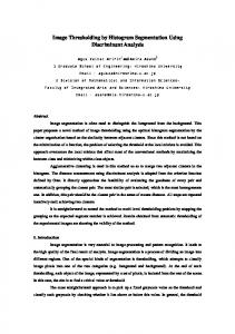
2 Analysis of the HSV Color Space A three dimensional representation of the HSV color space is a hexacone, with the central vertical axis representing intensity [11]. Hue is defined as an angle in the range [0,2π] relative to the red axis with red at angle 0, green at 2π/3, blue at 4π/3 and red again at 2π. Saturation is the depth or purity of color and is measured as a radial distance from the central axis with values between 0 at the center to 1 at the outer surface. For S=0, as one moves higher along the intensity axis, one goes from black to white through various shades of gray. On the other hand, for a given intensity and hue, if the saturation is changed from 0 to 1, the perceived color changes from a shade of gray to the most pure form of the color represented by its hue. Looked from a different angle, any color in the HSV space can be transformed to a shade of gray by sufficiently lowering the saturation. The value of intensity determines the particular gray shade to which this transformation converges. When saturation is near 0, all pixels, even with different hues, look alike and as we increase the saturation towards 1, they tend to get separated out and are visually perceived as the true colors represented by their hues. This is shown in Fig. 1(a). It is seen that the two leftmost circles in each row give similar impression of color to our eyes even though their hue values are quite different. This is due to low values of their saturation. For low saturation, a color can be approximated by a gray value specified by the intensity level while for higher saturation, the color can be approximated by its hue. The saturation threshold that determines this transition is once again dependent on the intensity. For low intensities, even for a high saturation, a color is close to the gray value and vice versa as shown in Fig. 1(b). In this figure, it is seen that although the saturation is 1.0 for each of the circles and their hue values are quite different, the leftmost circles in each row give similar impression of color to our eyes. This is due to low values of their intensity.

1(a)

1(b)

Fig. 1. Variation of color perception with (a) saturation (Decreasing from 1 to 0 right to left) for a fixed value of intensity and (b) intensity (Decreasing from 255 to 0 right to left) for a fixed value of saturation

Saturation gives an idea about the depth of color and human eye is less sensitive to its variation compared to variation in hue or intensity. We, therefore, use the saturation of a pixel to determine whether the hue or the intensity is more pertinent to human visual perception of the color of that pixel and ignore the actual value of the saturation. It is observed that for higher values of intensity, a saturation of about 0.2 differentiates between hue and intensity dominance. Assuming the maximum intensity value to be 255, we use the following threshold function to determine if a pixel should be represented by its hue or its intensity as its dominant feature. thsat(V) = 1.0 − 0.8V . 255

(1)

In the above equation, we see that for V=0, thsat(V) = 1.0, meaning that all the colors are approximated as black whatever be their hue or saturation. On the other hand, with increasing values of intensity, saturation threshold that separates hue dominance from intensity dominance goes down. Thus, we treat each pixel in an image either as a “true color” pixel – a pixel whose saturation is greater than thsat and hence, its hue is the dominant component or as a “gray color” pixel – a pixel whose saturation is less than thsat and hence, its intensity is the dominant component.

3 Segmentation using Saturation Thresholding 3.1 Feature Extraction We effectively use visual properties of the HSV color space as described in the last section for color image segmentation. Each image can be represented as a collection of its pixel features as follows: I≡{(pos, [t|g], val)} .

(2)

Here each pixel is a triplet where pos denotes the position of the pixel, [t|g] denotes whether the pixel is a “true color” pixel or a “gray color” pixel and val denotes the

“true color” value or the “gray color” value. Thus, val ∈[0,2π] if [t|g] takes a value of t and val ∈[0,255] if [t|g] takes a value of g. Essentially, we approximate each pixel either as a “true color” pixel or a “gray color” pixel with corresponding true/gray color values and then group similar “true color” or “gray color” values together to be represented by an average value for the group. In this approach, the feature of a pixel is the pair ([t|g], val) – whether it is a “true color” pixel or a “gray color” pixel and the corresponding hue or intensity value. Fig. 2(a) shows an original image and Fig. 2(b) shows the same image using the approximated pixels after saturation thresholding using Eq. (1). Pixels with sub-threshold saturation have been represented by their gray values while the other pixels have been represented by their hues. The feature generation method used by us makes an approximation of the color of each pixel in the form of thresholding. On the other hand, features generated from the RGB color space approximate by considering a few higher order bits only. In Figs. 2(c) - (d) we show the same image approximated with the six lower-order bits all set to 0 and all set to 1, respectively.

(a)

(b)

(c)

(d)

Fig. 2. (a) Original Image (b) HSV Approximation (c) RGB approximation with all low order bits set to 0 and (d) RGB approximation with all low order bits set to 1

It is seen that the approximation done by the RGB features blurs the distinction between two visually separable colors by changing the brightness. On the other hand, the proposed HSV-based approximation can determine the intensity and shade variations near the edges of an object, thereby sharpening the boundaries and retaining the color information of each pixel. 3.2 Pixel Grouping by K-means Clustering Algorithm Once we have extracted each pixel feature in the form of ([t|g],val), a clustering algorithm is used to group similar feature values. The clustering problem is to represent the image as a set of n non-overlapping partitions as follows: I ≡{O1|O2|O3|….|On} .

(3)

Here each Oi≡([t|g], val, {pos}), i.e., each partition represents either a “true color” value or a “gray color” value and it consists of the positions of all the image pixels that have colors close to val. We use K-Means clustering for pixel grouping. In the KMeans clustering algorithm, we start with K=2 and adaptively increase the number of clusters till the improvement in error falls below a threshold or a maximum number of clusters is reached. We set the maximum number of clusters to 12 and an error improvement threshold over number of clusters to 5 %.

3.3 Post Processing After initial K-Means clustering of image pixels, we get different color cluster centers and the image pixels that belong to these clusters. In Fig. 3(a), we show a natural scene image. In Fig. 3(b), we show the transformed image after feature extraction and K-Means clustering. It is observed that the clustering algorithm has determined five “true color” clusters, namely, Blue, Green, Orange, Yellow and Red for this particular image and three gray clusters – Black and two other shades of gray.

(a)

(b)

(c)

(d)

Fig. 3. Different Stages of Image Segmentation. (a) Original image (b) Image after clustering (c) Image after connected component analysis and (d) Final segmented image

However, these clustered pixels do not yet contain sufficient information about the various objects in the image. For example, it is not yet known if all the pixels that belong to the same cluster are actually part of the same object or not. To ascertain this, we next perform a connected component analysis [11] of the pixels belonging to each cluster. Connected component analysis is done separately for pixels belonging to each of the “true color” clusters and each of the “gray color” clusters. At the end of the connected component analysis step, we get the different objects of each color. During this process, we also identify the connected components whose size is less than a certain percentage (typically 1%) of the size of the image. These small regions are to be merged with the surrounding clusters in the next step. Such regions which are candidates for merger are shown in white in Fig. 3(c). In the last post-processing step, the small regions are merged with their surrounding regions with which they have maximum overlap. The image at the end of this step is shown in Fig. 3(d). It is seen that the various foreground and background objects of the image have been clearly segmented.

4 Web Based Image Retrieval Application We have developed a web-based CBIR application that matches images after segmenting them using the proposed method (www.imagedb.iitkgp.ernet.in/seg). A query in the application is specified by an example image. Initially, a random set of 20 images is displayed. Retrieval is done using the proposed feature extraction and segmentation approach with a suitable distance metric. The nearest neighbor result set is retrieved from the image database based on the query image and is displayed to the user. Users are often interested in retrieving images similar to their own query image. To facilitate this, we provide a utility to upload an external image file and use the image as a query on the database. We plan to enhance our application by displaying

the segmented image corresponding to the uploaded image as an extension of our work.

5 Results In this section, we show results of applying our segmentation method on different types of images. Figs. 4(a)-(c) show a number of original images, segmentation results using the proposed method and also the corresponding results of segmentation using the RGB color space.

(a)

(b)

(c)

Fig. 4. (a) Original Images (b) Segmentation using HSV features and (c) Segmentation using RGB features For RGB, we consider the higher order 2 bits to generate the feature vectors. In the images, we have painted the different regions using the color represented by the centroid of the clusters to give an idea about the differentiation capabilities of the two color spaces. Although exact segmentation of unconstrained color images is still a difficult problem, we see that the object boundaries can be identified in a way more similar to human perception of the same. The RGB features, on the other hand, fail to determine the color and intensity variations and come up with clusters that put neighboring pixels with similar color but small difference in shade to different clusters. Often, two distinct colors are merged together. In the HSV-based approach, better clustering was achieved in all the cases with proper segmentation. Fig. 5 shows some more examples of segmentation using the proposed approach that are considered difficult to segment using traditional methods.

Fig. 5. Segmentation results in the proposed system. The first image in each pair is the original image and the second is the segmented image 0.4 0.3 0.2 0.1 0

Precision

PP

1

0.5 0.1

0.3

0.5 0.7 Recall

6(a)

0.9

0 2

5

10

15

20 NN

6(b)

Fig. 6. (a) Precision vs. recall on a controlled database of 2,015 images. (b) Perceived precision variation on a large un-controlled database of 28,168 images

We first show the recall and precision of retrieval in our CBIR application on a controlled database of 2,015 images in Fig. 6(a). The database has various image categories, each containing between 20-150 images. Any image belonging to the same category as a query image is assumed to be a member of the relevant set. It should, however, be noted that the performance comparison of large contentbased image retrieval systems is a non-trivial task since it is very difficult to find the relevant sets for an uncontrolled database of general-purpose images. One way of presenting performance for such databases is through the use of a modified definition of precision. Even though we do not exactly know the relevant set, an observer’s perception of relevant images in the retrieved set is what can be used as a measure of precision. Thus, we re-define precision as “Perceived Precision” (PP) which is the percentage of retrieved images that are perceived as relevant in terms of content by the person running a query. By measuring PP of a large number of users and taking their mean, we get a meaningful representation of the performance of a CBIR system. In our experiments, we have calculated perceived precision for 50 randomly selected images of different contents and taken their average. Our database currently contains 28,168 images downloaded from the. PP is shown for the first 2, 5, 10, 15 and 20 nearest neighbors (NN) in Fig. 6(b). It is seen that the perceived precision stays almost constant from five to twenty nearest neighbors which implies that the number of false positives does not rise significantly as a larger number of nearest neighbors are considered.

6 Conclusions We have studied some of the important visual properties of the HSV color space and developed a framework for extracting features that can be used for effective image segmentation. Our approach makes use of the saturation value of a pixel to determine if the hue or the intensity of the pixel is more close to human perception of color that pixel represents. K-Means clustering of features is used to combine pixels with similar color for segmentation of the image into objects. A post-processing step filters out small extraneous clusters to identify correct object boundaries in the image. An image retrieval system has been developed in which database images are ranked based on their distance from a query image. Promising retrieval results are obtained even for a large database of about 28,000 images. We plan to increase the database size to about 80,000 images and compare our results with other segmentation-based retrieval systems.

Acknowledgement The work done by Shamik Sural is supported by research grants from the Department of Science and Technology, India, under Grant No. SR/FTP/ETA-20/2003 and by a grant from IIT Kharagpur under ISIRD scheme No. IIT/SRIC/ISIRD/2002-2003.

References 1.

Carson, C. et al: Blobworld: A System for Region-based Image Indexing and Retrieval. Third Int. Conf. on Visual Information Systems, June (1999) 2. Chen, J., Pappas, T.N., Mojsilovic, A., Rogowitz, B.: Adaptive Image Segmentation Based on Color and Texture. IEEE Conf. on Image Processing (2002) 3. Deng, Y., Manjunath, B.S.: Unsupervised Segmentation of Color-texture Regions in Image and video. IEEE Trans. on PAMI, Vol. 23 (2001) 800-810 4. Kaufman, L., Rousseeuw, P.J.: Finding Groups in Data: An Introduction to Cluster Analysis. John Wiley & Sons, New York (1990) 5. Ma, W.Y., Manjunath, B.S.: NeTra: A Toolbox for Navigating Large Image Databases. IEEE Int. Conf. on Image Processing (1997) 568-571 6. Niblack W. et al: The QBIC Project: Querying Images by Content using Color Texture and Shape. SPIE Int. Soc. Opt. Eng., In Storage and Retrieval for Image and Video Databases, Vol. 1908, (1993) 173-187 7. Ortega, M. et al: Supporting Ranked Boolean Similarity Queries in MARS. IEEE Trans. on Knowledge and Data Engineering, Vol. 10 (1998) 905-925 8. Randen, T., Husoy, J.H.: Texture Segmentation using Filters with Optimized Energy Separation. IEEE Trans. on Image Processing, Vol. 8 (1999) 571–582 9. Smeulders, A.W.M. et al: Content Based Image Retrieval at the End of the Early Years. IEEE Trans. on PAMI, Vol. 22 (2000) 1-32 10. Smith, J.R., Chang, S.-F.: VisualSeek: A Fully Automated Content based Image Query System. ACM Multimedia Conf., Boston, MA (1996) 11. Stockman, G., Shapiro, L.: Computer Vision. Prentice Hall, New Jersey (2001) 12. Wang, J.Z., Li, J., Wiederhold, G.: SIMPLIcity: Semantics-sensitive Integrated Matching for Picture Libraries. IEEE Trans. on PAMI, Vol. 23 (2001).