Multiobjective Programming and Multiattribute Utility Functions in Portfolio Optimization Matthias Ehrgott, Chris Waters Department of Engineering Science The University of Auckland Private Bag 92019, Auckland, New Zealand email:
[email protected] Rafail N. Gasimov, Ozden Ustun Department of Industrial Engineering Osmangazi University Bademlik 26030, Eski¸sehir, Turkey email: {gasimovr,
[email protected]} August 14, 2006 Abstract In recent years portfolio optimization models that consider more criteria than the standard expected return and variance objectives of the Markowitz model have become popular. For such models, two approaches to find a suitable portfolio for an individual investor are possible. In the multiattribute utility theory (MAUT) approach a utility function is constructed based on the investor’s preferences and an optimization problem is solved to find a portfolio that maximizes the utility function. In the multiobjective programming (MOP) approach a set of efficient portfolios is computed by optimizing a scalarized objective function. The investor then chooses a portfolio from the efficient set. We outline these two approaches using the UTADIS method to construct a utility function and present numerical results for an example. Keywords: Portfolio optimization; multiobjective programming; multiattribute utility function; UTADIS.
1
Portfolio Optimization
Multicriteria portfolio optimization started with the Markowitz mean-variance model (Markowitz, 1952, 1959). This model assumes that the goal of an average or standard investor is to maximize the (unknown and uncertain) return on investment. The mean-variance model is one possible deterministic substitute of this stochastic optimization problem with the objective to maximize the expected return subject to a constraint on its variance. Let n be the number of available assets, let xi and ri be the fraction of the available capital invested in and the expected return, respectively of asset i for i = 1, . . . , n. Let and σij be the covariance of the returns of assets i and j. The optimization problem considered in the Markowitz model is then
1
max f1 (x) =
n X
ri xi
i=1
subject to f2 (x) =
n X n X
≤
ε
xi
=
1
xi
≥
0 for all i = 1, . . . , n.
σij xi xj
(1)
i=1 j=1
n X i=1
If σmin and σmax are the minimal and maximal attainable values of f2 (x) it is easy to see that all x that maximize (1) for some ε ∈ [σmin , σmax ] are contained in the set of (weakly) efficient solutions of the biobjective optimization problem max f1 (x)
=
min f2 (x)
=
n X
ri xi i=1 n X n X
σij xi xj
(2)
i=1 j=1
n X
xi
= 1
xi
≥ 0 for all i = 1, . . . , n.
i=1
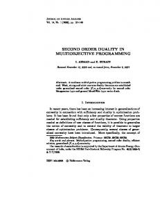
An efficient solution of (2) is a portfolio, which has the property that when moving to a portfolio with higher return variance will also increase, and when moving to a portfolio with smaller variance, return will decrease, too. Clearly, non-efficient portfolios are undesirable in this context and every efficient portfolio is also an optimal solution to (1) with ε = f2 (x). The non-dominated frontier consists of all possible combinations of expected returns and variances of efficient portfolios. Figure 1 shows the (approximated) non-dominated frontier for an example with n = 40 assets. This figure is for the data set we will use throughout the paper. 350 300 250
f1
200 150 100 50 0 0
200
400
600
800 f2
1000
1200
1400
1600
Figure 1: Approximated efficient frontier for an example with n = 40. While the Markowitz model permeates the field of finance until today, there has been an increasing number of publications that suggest that it is not always appropriate, at least in the case of individual rather than standard investors. We mention a few such publications, but refer to Steuer and Na (2003) for a more detailed analysis of the literature. 2
Arthur and Ghandforoush (1987) suggest that there are objective and subjective measures for portfolios. Konno (1990) observes that most investors do not actually buy efficient portfolios, but rather those behind the nondominated frontier. Ballestero and Romero (1996) argue for a need to modify the model for average investors in order to approximate the optimal portfolio of an individual investor. Hallerbach and Spronk (1997) explain that most models do not incorporate the multidimensional nature of the problem and outline a framework for such a view on portfolio management. Finally, Steuer et al. (2006) introduce the “suitable portfolio” investor, who may include objectives other than expected return and variance in their portfolio selection problem. They also explain the fact that investors do buy non-efficient portfolios as the effect of projecting the multidimensional space of the individual investor’s portfolio selection problem to the two-dimensional mean-variance space: The selected portfolios are actually efficient in the higher dimensional space. In this paper, we have chosen one exemplary multiobjective model of portfolio optimization to illustrate the two approaches to portfolio selection. This is the model presented in Ehrgott et al. (2004), which we can consider as a particular investor’s portfolio selection problem. The five criteria of this model include 12-month performance, 3-year performance, and annual dividend as measures of return. The fourth objective is the Standard and Poor’s star ranking, which describes to what extent an investment fund follows a specific market index and is applied particularly in the case that a portfolio consists exclusively of investment funds, which is the case for the data set we use for numerical experiments. The fifth attribute, the 12-month variance, is used as a measure of the risk of a portfolio. For asset i ∈ {1, . . . , n} let ri12 be the 12-month performance (expected return), let ri36 be the 36-month (long term) performance, let di ≥ 0 be the relative annual dividend, and let si ∈ {1, 2, 3, 4, 5} be the number of stars assigned to asset i (one star indicates relatively poor performance of assets and five stars indicate very good performance). Furthermore let σij be the covariance between the returns of assets i and j. We define the following five objective functions. Pn • f1 (x) = i=1 ri12 xi is the 12-month performance. This objective function is a measure for the short term expected return. Pn • f2 (x) = i=1 ri36 xi , the 3-year performance, is a measure for the long term expected return. P • f3 (x) = ni=1 di xi represents the relative annual dividend of a portfolio. P • f4 (x) = ni=1 si xi is the average star ranking of portfolio x. Standard and Poor’s Fund Service GmbH evaluates the performance of most investment funds contained in their data base on an annual basis which results in a performance ranking. Pn Pn • f5 (x) = − i=1 j=1 σij xi xj is the usual variance measure of portfolio risk (we take the negative value so as to maximize all objectives). Thus, our multiobjective portfolio optimization problem can be written as follows: max(f1 (x), . . . , f4 (x), f5 (x)) n X subject to xi
=
1
≥
0 for all i = 1, . . . , n.
(3)
i=1
xi
In addition to replacing the two objectives of the Markowitz model (2) by five, we include additional constraints on the minimal and maximal fraction of the capital that can be invested in a single asset and on the number of assets in the portfolio (see also Chang et al. (2000)). For that purpose let yi , i = 1, . . . , n denote binary variables with yi = 1 if and only if asset i is contained in the portfolio. With these additions the problem we consider in this paper is
3
max(f1 (x), . . . , f4 (x), f5 (x)) n X subject to xi
=
1
yi
=
k
xi xi
≤ ≥
ri yi for all i = 1, . . . , n li yi for all i = 1, . . . , n
xi yi
≥ ∈
0 for all i = 1, . . . , n {0, 1} for all i = 1, . . . , n.
i=1 n X
(4)
i=1
The goal of portfolio selection is of course to find the most suitable portfolio for our individual investor. To be able to do this, we have to assume the existence of a utility function for the investor: The utility of a portfolio is a (real-valued) function of the portfolio’s score on the five criteria specified above. It is important to note that this utility function is usually not explicitly available. The most suitable portfolio is then the one with the highest utility. To compute it there are two possible strategies. In the multiobjective programming approach, we find a set of efficient solutions of (4). The multiattribute utility theory approach is to elicit information from the investor that allows the construction of a utility function. This is then used to convert (4) into a single objective optimization problem which is solved directly to obtain the portfolio with maximal utility. The two strategies are presented in Sections 2 and 3. In Section 4 we present the results of numerical tests on a dataset with n = 40 sets obtained from the Standard and Poor’s database in 1999.
2
Multiobjective Programming
In this section we introduce some definitions and results of multiobjective programming. A multiobjective programming problem can be written as max f (x), x∈X
(5)
where X ⊂ Rn is the feasible set in decision space Rn and f : Rn → Rp is a vector valued objective function mapping a feasible solution x to a point f (x) = (f1 (x), . . . , fp (x)) in objective space Rp . We denote by Y := f (X) the feasible set in objective space. Let Rp= := {y ∈ Rp : yk = 0, k = 1, . . . , p} and Rp> := {y ∈ Rp : yk > 0, k = 1, . . . , p}. For any y 1 , y 2 ∈ Rp we define y1
5 y 2 if y 2 − y 1 ∈ Rp= ,
y1
≤ y 2 if y 1 5 y 2 and y 1 6= y 2 ,
y1
< y 2 if y 2 − y 1 ∈ int Rp= = Rp> .
In the context of portfolio optimization we will have X = {(x, y) ∈ Rn= × {0, 1}n : eT x = 1; li yi ≤ xi ≤ ri yi for i = 1, . . . , n}. Definition 1 Let Y be a non-empty subset of Rp . 1. An element y ∈ Y is called non-dominated if ({y} + Rp= ) ∩ Y = {y}, i.e. there is no y 0 ∈ Y such that y 0 ≥ y.
4
2. An element y ∈ Y is called properly non-dominated (in the sense of Benson) if y is a non-dominated element of Y and the zero element of Rp is a non-dominated element of p cl cone(Y − R= − y), where cl(Y ) denotes the closure of a set Y and cone(Y ) := {αy : α ≥ 0, y ∈ Y }. The set of all non-dominated elements of Y is denoted YN , the set of all properly non-dominated elements YpN . Definition 2 A feasible solution x ∈ X is called (properly) efficient if y = f (x) is a (properly) non-dominated element of Y . The set of (properly) efficient solutions of a multiobjective programming problem is denoted XE (XpE ). Multiobjective programming problems are generally solved through scalarization. The multiobjective programme (5) is transformed into a single objective problem minx∈X s(x, λ), the objective function of which depends on parameter λ. Solving the single objective problem for a range of parameter values yields (some) efficient solutions to the multiobjective programme. Many scalarization methods are known, see the survey in Ehrgott and Wiecek (2005). The main issues for solving a multiobjective programme by scalarization are to show that a) every optimal solution to the scalarized problem is efficient and b) for every efficient solution x ˆ to a multiobjective ˆ ˆ programme there is a parameter λ such that x ˆ is an optimal solution to minx∈X s(x, λ). In this paper we use the scalarization of Gasimov (2001). He introduces a class of increasing convex functions to scalarize the multiobjective programme (5) without any assumptions on objectives and constraints of the problem under consideration. Another advantage of this approach is that it preserves convexity, if the objective functions of the initial problem are linear or convex. Now we briefly present the main scalarization results of Gasimov (2001). Let n o W := (α, w) ∈ R × Rp= : 0 ≤ α < min{w1 , . . . , wp } . (6) Theorem 1 (Gasimov (2001)) Suppose that for some (α, w) ∈ W a feasible solution x ˆ ∈ X is an optimal solution to the scalar maximization problem ! p p X X max α |fk (x)| + wk fk (x) . (7) x∈X
k=1
k=1
then x ˆ is a Benson properly efficient solution to (5). Theorem 2 (Gasimov (2001)) Let x ˆ ∈ X be a Benson proper efficient solution to (5). Then there exists a vector (α, w) ∈ W such that x ˆ is an optimal solution to the scalar maximization problem p 1 X X |fk (x) − fk (ˆ x)| + wk (fk (x) − fk (ˆ x)) (8) max α x∈X
k=1
k=1
In non-convex multiobjective programmes the distinction between supported and non-supported efficient solutions is important. An efficient solution xˆ ∈ XE is called supported, if there is w ∈ Rp> such that x ˆ is an optimal solution to max x∈X
p X
wk fk (x).
k=1
It is well known (Geoffrion, 1968) that if X is convex and all fk , k = 1, . . . , p are convex functions, then all Benson proper efficient solutions are supported, see e.g. Ehrgott (2005). However, for non-convex problems there exist non-supported efficient solutions. This observation yields the following Lemma. 5
Lemma 1 Let Y ⊂ Rp be a non-empty set, P let yˆ ∈ Y be a non-dominated Pppoint of Y , and let p y 1 , . . . , y m ∈ Y . If there is some β ∈ Rp> with k=1 βk = 1 such that y β = k=1 βk yk < yˆ then yˆ is not an optimal solution to the weighted sum problem maxy∈Y λT y, where λ ∈ Rp> . It is evident that if x ˆ ∈ X is an efficient solution to problem (5) then it is also an efficient solution to the shifted multiobjective programme max(f1 (x) − a1 , . . . , fp (x) − ap ),
(9)
x∈X
where a ∈ Rp is an arbitrary vector. Such a shifting can be used in situations when objectives do not change sign on the whole feasible set X in order to make the absolute value used in the scalarized problem (7) sensible. In this case we can formulate the following scalarized problem, which is similar to that in (8), and can be used even if we do not know any efficient solution. ! p p X X wk (fk (x) − ak ) . (10) |fk (x) − ak | + max α x∈X
k=1
k=1
We can therefore completely characterize Benson proper efficient solutions through Gasimov’s scalarization. Corollary 1 A feasible solution x ˆ ∈ X is Benson proper efficient if and only if there are a ∈ Rp , p α ∈ R, and w ∈ R= with (α, w) ∈ W such that x ˆ is an optimal solution to max α x∈X
p X
|fk (x) − ak | +
k=1
p X
!
wk (fk (x) − ak ) .
k=1
Note that for α = 0 (11) reduces to the weighted sum scalarization maxx∈X Therefore non-supported efficient solutions can only be found with α > 0.
3
(11) Pp
k=1
wk fk (x).
Multiattribute Utility Theory and the UTADIS Method
In the multiattribute utility theory (MAUT) approach to portfolio optimization the goal is to construct a utility function, that assigns any portfolio x ∈ X a utility value. The utility function is a function of the scores of a portfolio on the selected criteria or attributes. The portfolio optimization problem is then solved by finding a portfolio that maximizes the utility function. According to Keeney and Raiffa (1993) the set of attributes should be complete, operational, decomposable, non-redundant, and minimal. It is well known that an additive utility function exists if the attributes are mutually preferentially independent Keeney and Raiffa (1993). This means that the conditional preferences of one attribute given a second attribute do not depend on the value of the second attribute. We shall assume that an additive utility function exists. Thus, we assume that there is a function U : Rp → R that maps an outcome vector y ∈ Rp to a global utility value U (y) ∈ R. U has the form U (y) =
p X
µk u ˜k (yk ),
(12)
k=1
where the marginal utility functions u ˜k satisfy 0 ≤ u ˜k (yk ) ≤ 1 for all y ∈ Y and k = 1, . . . , p and µk is an importance weight of marginal utility function u˜k . In this section we explain how to construct U using the UTADIS method as described in Doumpos and Zopounidis (2002). The UTADIS method (Utilit´es Additives Discriminates) is a method developed for the classification of a finite set of alternatives xj with attribute vectors y j into q predefined ordered classes Cl , where C1 and Cq contain the most and least preferred alternatives, respectively. This is done by constructing an additive utility function U as in (12) and 6
utility thresholds u ¯l ∈ R for l = 1, . . . , q−1 such that xj is assigned to class Cl if u ¯l ≤ U (y j ) < u ¯l−1 (here u¯0 = ∞ and u ¯q = −∞). A reference set {xj : j = 1, . . . , o} of alternatives is selected and classified into the q classes according to the values ykj = fk (xj ) by the decision maker. We denote by ml the number of alternatives of the reference set in class Cl . An optimization model is then formulated to determine the marginal utility functions u ˜k , their weights µk and the utility thresholds u¯l . The objective of this optimization problem is the minimization of the classification error rate on the reference set. If the marginal utilities u ˜k are approximated by piecewise linear functions, the optimization problem turns into a linear programme. For ease of exposition we assume now that all u˜k are increasing, i.e. more is preferred to less for all attributes yk , and let [yk∗ , yk∗ ] be the possible range of values. To further simplify notation, we let uk = µk u ˜k (so that µk = uk (yk∗ ) and uk (yk∗ ) = 0). For each of the p criteria yk , let h yk , h = 1, . . . , hk denote the breakpoints of the piecewise linear function uk with yk1 = yk∗ and ykhk = yk∗ . Then h−1 X yk − y h uk (yk ) = wkr + h+1 k h wkh0k yk − yk r=1
for all yk ∈ [ykh , ykh+1 ] and appropriately chosen constants wkr = uk (ykh+1 ) − uk (y h ). The global utility of an alternative x with criteria or attribute vector y = f (x) is then 0 hk −1 p h0k X X y − y k U (y) = wkr + h0 +1 k h0 wkh0k , k yk − yk k r=1 k=1 h0
h0 +1
where h0k denotes the interval [yk k , yk k ] in which the value yk falls. Letting σj+ := max{0, u ¯l − U (y j )} and σj− := max{0, U (y j ) − u ¯l−1 } for y ∈ Cl , l = 1, . . . , q be j the classification errors for alternative x in the reference set, we can formulate the LP q X 1 X + min (σj + σj− ) ml j l=1 x ∈Cl 0 0 hk −1 p hk j X X y − y wkr + h0 k+1 k h0 wkh0k − u¯1 + σj+ yk k − yk k r=1 k=1 0 hk −1 p h0k j X X y − y ¯l + σj+ wkr + h0 k+1 k h0 wkh0k − u k k − y y r=1 k=1 k k 0 0 hk −1 p h j k X X y − y wkr + h0 k+1 k h0 wkh0k − u¯l−1 − σj− yk k − yk k r=1 k=1 0 hk −1 p h0k j X X y −y ¯q−1 − σj− wkr + h0 k+1 k h0 wkh0k − u k k yk − yk r=1 k=1
(13)
≥
δ1
xj ∈ C1
(14)
≥
δ1
xj ∈ Cl , 2 ≤ l ≤ q − 1
(15)
≤
−δ2
xj ∈ Cl , 2 ≤ l ≤ q − 1
(16)
≤
−δ2
xj ∈ Cq
(17)
wkh
=
1
u ¯l − u ¯l+1
≥
s
σj+ , σj−
≥ ≥
0 j = 1, . . . , o 0 k = 1, . . . , p
p hX k −1 X
(18)
k=1 h=1
wkh
l = 1, . . . , q − 2
h = 1, . . . , hk − 1
7
(19) (20) (21)
Constraints (14) – (17) define the classification errors σj+ and σj− . (18) normalizes the utility function U so that U (y ∗ ) = 1, (19) makes sure that utility thresholds are different. The parameters δ1 and δ2 are small positive numbers to avoid cases where U (y j ) = u¯k for xj ∈ Cl . s is chosen to be bigger than δ1 and δ2 and guarantees that u¯l+1 is greater than u ¯l . The variables in the LP are wkr , u ¯l , and σj+ , σj− . The utility function U (y) was used to formulate a mixed integer non-linear programme max U (f (x))
=
5 X
µk u˜k (fk (x))
k=1
subject to
n X
i=1 n X
xi
=
1
yi
=
k
xi
≤
ri yi for all i = 1, . . . , n
xi xi
≥ ≥
li yi for all i = 1, . . . , n 0 for all i = 1, . . . , n
yi
∈
{0, 1} for all i = 1, . . . , n.
(22)
i=1
We address the question, whether an optimal solution of (22) is an efficient solution to (4). Proposition 1 Let U : Rp → R be componentwise increasing and assume that U attains its maximum at y ∗ . Then y ∗ is a non-dominated element of Y . Proof: Let U (y ∗ ) = max{U (y) : y ∈ Y }. If y ∗ is dominated there exists some y ∈ Y such that yk ≥ yk∗ for all k = 1, . . . , p and yj > yj∗ for at least one index j. Because U is componentwise increasing, we have U (y) > U (y ∗ ), a contradiction that implies that y ∗ is nondominated. 2 Note that the function U used in (22) is componentwise increasing because the marginal utility functions u ˜k are all increasing. Then the fact that YN = f (XE ) implies that an optimal solution of (22) is an efficient solution of (4). We also want to study the effect of the cardinality of the portfolio on its utility. That can be done by solving (22) for all feasible values of k. In order to obtain the portfolio with maximal utility, independent of the cardinality, but with the lower and upper bounds on xi , we remove the Pn constraint i=1 yi = k.
4
Results
We have used a dataset of n = 40 investment funds from Standard and Poor’s 1999 database. For the numerical tests we have considered an unconstrained problem (i.e. the number of assets in the portfolio was not prescribed and all lower bounds li = 0, all upper bounds ri = 1) as well as a constrained problem with the values li = 0.05, ri = 0.3 to limit the fraction of an asset in a portfolio and k = 10 for cardinality constrained portfolios. For both problems we have solved the scalarized MOP (11) and the non-linear (mixed integer) problem (22). All problems were solved using the GAMS/MINOS derivative-free nonlinear programming (DNLP) solver and GAMS/DICOPT mixed integer nonlinear programming (MINLP) solver. Documentation and information about GAMS and its solvers are available on the Internet at www.gams.com. All programs have been run on a HP Workstation xw6000 with WINDOWS operating system on two processors. For the unconstrained portfolio problem we have used a = (234.46, 175.3, 4.51, 3, 0) and various values of α and w in (11) to find efficient solutions to problem (3) corresponding to some nondominated points. The non-dominated points are presented in Table 1.
8
Table 1: Non-dominated points of the unconstrained problem found by solving (10). No.
α
w1
w2
w3
w4
w5
f1
f2
f3
f4
f5
1 2 3 4 5 6 7 8 9 10 11 12 13 14 15 16 17 18 19 20 21 22 23 24 25 26 27 28 29 30 31 32 33 34 35 36 37 38 39 40 41 42 43 44 45 46 47
0 0 0 0 0 0 0 0 0 0 0 0 0 0 0 0 0 0 0 0 4 5 1 4 1 4 3 1 2 3 1 10 1 2 0 5 4 4 5 1 1 1 1 1 1 1 0.25
1 0 0 0 0 1 1 1 1 1 1 4 5 1 1 1 1 250 1000 1 4 9 1 12 8 10 3 5 5 6 20 21 1 20 2 5 4 4 5 1 1 1000 1 1 1 1 16.27
0 1 0 0 0 1 1 1 1 1 1 6 5 1 1 1 1 250 5000 2 5 8 1 11 8 5 4 1 2 9 50 51 10 5 10 15 8 6 5 1 1 1 1000 1 1 1 0.25
0 0 1 0 0 1 1 1 1 1 1 30 30 2 5 1000 250 5000 250 1 6 7 1 10 8 10 5 2 2 9 20 21 10 4 10 15 16 30 30 2 5 1 1 1000 1 1 3.21
0 0 0 1 0 1 1 1 1 1 1 30 5 1000 2000 1000 750 250 1000 2 7 6 1 9 8 5 3 3 3 9 50 51 1 3 10 5 32 30 30 1000 2000 1 1 1 1000 1 53.52
0 0 0 0 1 1 5 10 20 50 1000 30 5 2000 6000 1000 1000 5000 1000 1 8 5 1 8 2 10 4 4 4 9 20 21 50 2 100 5 64 30 5 2000 6000 1 1 1 1 1000 26.75
432.89 234.46 11.40 15.96 97.19 432.89 432.89 432.89 432.89 432.89 275.68 432.89 432.89 82.73 83.17 0.90 20.16 432.89 432.89 432.89 308.02 432.89 234.48 432.89 432.89 432.89 287.52 432.89 432.89 432.89 432.89 432.89 274.21 432.89 432.89 234.46 315.78 315.78 234.47 114.36 90.08 432.89 234.46 11.40 153.12 234.46 432.89
333.20 336.49 37.64 57.69 124.39 333.20 333.20 333.20 333.20 333.20 261.98 333.20 333.20 119.54 116.76 24.55 88.79 333.20 333.20 333.20 335.27 333.20 193.91 333.20 333.20 333.20 335.61 333.20 333.20 333.20 333.20 333.20 335.83 333.20 333.20 336.49 335.14 335.14 194.08 156.87 128.44 333.20 336.49 37.64 175.77 218.40 333.20
0.00 0.00 8.55 2.93 1.87 0.00 0.00 0.00 0.00 0.00 0.11 0.00 0.00 0.47 0.45 5.34 4.73 0.00 0.00 0.00 0.00 0.00 3.93 0.00 0.00 0.00 0.00 0.00 0.00 0.00 0.00 0.00 0.00 0.00 0.00 0.00 0.00 0.00 4.02 0.56 0.43 0.00 0.00 8.55 0.00 0.18 0.00
4.00 4.00 1.00 5.00 2.83 4.00 4.00 4.00 4.00 4.00 4.07 4.00 4.00 5.00 4.98 5.00 5.00 4.00 4.00 4.00 4.00 4.00 2.70 4.00 4.00 4.00 4.00 4.00 4.00 4.00 4.00 4.00 4.00 4.00 4.00 4.00 4.00 4.00 2.59 4.89 4.94 4.00 4.00 1.00 5.00 3.85 4.00
1.00 1.00 1.00 0.83 0.39 1.00 1.00 1.00 1.00 1.00 0.58 1.00 1.00 0.54 0.53 1.00 0.77 1.00 1.00 1.00 0.78 1.00 0.76 1.00 1.00 1.00 0.82 1.00 1.00 1.00 1.00 1.00 0.86 1.00 1.00 1.00 0.77 0.77 0.76 0.57 0.52 1.00 1.00 1.00 1.00 0.51 1.00
9
In Table 2 eleven efficient solutions obtained for nonzero values of the parameter α extracted from Table 1 are presented. As it can be seen from Table 2 different efficient solutions have been obtained for the cases α = 0 and α 6= 0. It is remarkable that the conic scalarization method provides different solutions for the same set of preference weights, while very similar solutions have been calculated for different weights with α = 0. Table 2: Non-dominated points of the unconstrained problem found by solving (10) with zero and nonzero α. No. α w1 w2 w3 w4 w5 f1 f2 f3 f4 f5 21 23 27 33 37 38 39 40 41 45 46
4 0 1 0 3 0 1 0 4 0 4 0 5 0 1 0 1 0 1 0 1 0
4 4 1 1 3 3 1 1 4 4 4 4 5 5 1 1 1 1 1 1 1 1
5 5 1 1 4 4 10 10 8 8 6 6 5 5 1 1 1 1 1 1 1 1
6 6 1 1 5 5 10 10 16 16 30 30 30 30 2 2 5 5 1 1 1 1
7 7 1 1 3 3 1 1 32 32 30 30 30 30 1000 1000 2000 2000 1000 1000 1 1
8 8 1 1 4 4 50 50 64 64 30 30 5 5 2000 2000 6000 6000 1 1 1000 1000
308.02 432.89 234.48 432.89 287.52 432.89 274.21 432.89 315.78 432.89 315.78 432.89 234.47 432.89 114.36 82.73 90.08 83.17 153.12 152.86 234.46 275.68
335.27 333.20 193.91 333.20 335.61 333.20 335.83 333.20 335.14 333.20 335.14 333.20 194.08 333.20 156.87 119.54 128.44 116.76 175.77 176.94 218.40 261.98
0.00 0.00 3.93 0.00 0.00 0.00 0.00 0.00 0.00 0.00 0.00 0.00 4.02 0.00 0.56 0.47 0.43 0.45 0.00 0.00 0.18 0.11
4.00 4.00 2.70 4.00 4.00 4.00 4.00 4.00 4.00 4.00 4.00 4.00 2.59 4.00 4.89 5.00 4.94 4.98 5.00 5.00 3.85 4.07
In Table 3 we show non-dominated points obtained for the constrained problem (4).
10
0.78 1.00 0.76 1.00 0.82 1.00 0.86 1.00 0.77 1.00 0.77 1.00 0.76 1.00 0.57 0.54 0.52 0.53 1.00 1.00 0.51 0.58
Table 3: Non-dominated points of the constrained problem found by solving (10). No.
α
w1
w2
w3
w4
w5
f1
f2
f3
f4
f5
1 2 3 4 5 6 7 8 9 10 11 12 13 14 15 16 17 18 19 20 21 22 23 24 25 26 27 28 29 30 31 32 33 34 35 36 37 38 39 40 41 42 43 44 45 46 47
0 0 0 0 0 0 0 0 0 0 0 0 0 0 0 0 0 0 0 0 4 5 1 4 1 4 3 1 2 3 1 10 1 2 0 5 4 4 5 1 1 1 1 1 1 1 0.25
1 0 0 0 0 1 1 1 1 1 1 4 5 1 1 1 1 250 1000 1 4 9 1 12 8 10 3 5 5 6 20 21 1 20 2 5 4 4 5 1 1 1000 1 1 1 1 16.27
0 1 0 0 0 1 1 1 1 1 1 6 5 1 1 1 1 250 5000 2 5 8 1 11 8 5 4 1 2 9 50 51 10 5 10 15 8 6 5 1 1 1 1000 1 1 1 0.25
0 0 1 0 0 1 1 1 1 1 1 30 30 2 5 1000 250 5000 250 1 6 7 1 10 8 10 5 2 2 9 20 21 10 4 10 15 16 30 30 2 5 1 1 1000 1 1 3.21
0 0 0 1 0 1 1 1 1 1 1 30 5 1000 2000 1000 750 250 1000 2 7 6 1 9 8 5 3 3 3 9 50 51 1 3 10 5 32 30 30 1000 2000 1 1 1 1000 1 53.52
0 0 0 0 1 1 5 10 20 50 1000 30 5 2000 6000 1000 1000 5000 1000 1 8 5 1 8 2 10 4 4 4 9 20 21 50 2 100 5 64 30 5 2000 6000 1 1 1 1 1000 26.75
280.02 243.00 17.64 45.31 97.98 272.96 272.96 272.96 270.77 259.04 233.22 252.73 272.96 82.33 86.54 22.06 53.13 270.67 247.30 252.73 241.78 272.96 234.46 272.96 272.96 278.96 241.78 280.02 280.02 252.73 247.30 247.30 241.78 278.96 247.3 241.78 241.78 241.09 234.46 148.25 88.84 280.02 243.00 25.93 139.46 234.46 280.02
240.80 278.80 43.09 133.97 127.38 258.01 258.01 258.01 259.93 270.27 240.88 275.84 258.01 120.03 127.54 65.35 114.57 256.81 278.15 275.84 278.52 258.01 210.38 258.01 258.01 247.32 278.52 240.80 240.80 275.84 278.15 278.15 278.52 247.32 278.15 278.52 278.52 277.79 217.31 175.3 130.92 240.80 278.80 73.81 160.22 218.58 240.80
0.29 0.35 5.94 2.11 1.41 0.35 0.35 0.35 0.35 0.35 0.20 0.35 0.35 0.81 0.56 5.47 3.04 0.58 0.37 0.35 0.60 0.35 2.29 0.35 0.35 0.37 0.60 0.29 0.29 0.35 0.37 0.37 0.60 0.37 0.37 0.60 0.60 0.64 2.19 0.75 0.56 0.29 0.35 5.92 0.55 0.54 0.29
4.15 4.25 2.40 5.00 3.11 4.30 4.30 4.30 4.30 4.30 4.02 4.30 4.30 5.00 4.95 3.50 5.00 4.20 4.25 4.30 4.15 4.30 3.52 4.30 4.30 4.20 4.15 4.15 4.15 4.30 4.25 4.25 4.15 4.20 4.25 4.15 4.15 4.20 3.70 4.78 4.94 4.15 4.25 2.40 4.95 3.80 4.15
0.73 0.67 0.79 0.81 0.39 0.71 0.71 0.71 0.69 0.64 0.53 0.63 0.71 0.54 0.53 0.76 0.64 0.70 0.64 0.63 0.67 0.71 0.65 0.71 0.71 0.72 0.67 0.73 0.73 0.63 0.64 0.64 0.67 0.72 0.64 0.67 0.67 0.67 0.67 0.52 0.52 0.73 0.67 0.68 0.72 0.53 0.73
11
For the multiattribute utility model (22) we have to discuss the assumptions first. We have to mention that our five attributes do probably not entirely satisfy the decomposability and nonredundancy (12-month and 3-year performance are certainly correlated to some extent and the Standard & Poor’s star ranking measures both risk and return), this was accepted for this study. We are also aware of the fact that due to correlation among some of the attributes mutual preferential independence is probably not completely satisfied. Nevertheless, we assume that an additive utility function exists for this problem. We have used the set of single asset portfolios as reference set, i.e. xj = ej , where ej is the th j unit vector in Rn and three classes, i.e. q = 3. The classification of the reference set was done by one of the authors (Waters). The breakpoints ykh were chosen such that, after ranking the alternatives according to criterion k, an equal number of alternatives would fall into each interval [ykh , ykh+1 ]. We chose hk = 6, i.e. 5 intervals for each criterion and chose the parameters δ1 = δ2 = 0.0001 and s = 2δ1 . After solving LP (13) – (21) we have also performed sensitivity analysis as recommended in Doumpos and Zopounidis (2002). This involved solving additional LPs with the objective to minimize the utility thresholds u ¯l and the weights µk of the objectives, respectively, with a constraint that the classification error is at most 5% worse than in the original LP (13) – (21). The solutions of all LPs were very similar. We have averaged the results to obtain the final utility function U . The details are given in Table 4. Table 4: Breakpoints ykh and weights µk of utility functions u ˜k . 12-month yk u ˜k 0 15 40 60 150 450 µk
0.000 3.966 3.966 3.966 3.966 100.000 16.27
3-year yk
u˜k
0 40 90 130 180 350
0.000 97.558 100.000 100.000 100.000 100.000
Dividend yk u ˜k 0.0 0.5 1.5 2.5 4.5 10.0
0.25
0.000 1.651 16.350 16.835 16.835 100.000
Variance yk
u ˜k
0 5 15 20 30 50
100.000 96.632 96.584 95.672 90.207 0.000
3.21
26.75
Star Ranking yk u ˜k 0 2 3 4 5
0.000 98.671 98.671 99.706 100.000 53.52
The piecewise linear utility functions uk were implemented as follows. Let yk1 , . . . , ykhk be the breakpoints. Then yk = ykh zh + ykh+1 (1 − zh ) for some 0 ≤ zh ≤ 1 and ykh ≤ yk ≤ ykh+1 . Thus uk (yk ) = uk (ykh )zh + uk (ykh+1 )(1 − zh ) and the piecewise linear function uk is modeled by adding the constraints zh
≤
wh−1 + wh
wh
=
1
zh
=
1
ykh zh
=
yk
wh zh
∈ ≥
{0, 1} h = 1, . . . , hk 0 h = 1, . . . , hk
hk X
h = 1, . . . , hk
h=1 hk X
h=1 hk X
h=1
with w0 = whk = 0. 12
Table 5: Points of the constrained problem found by solving (22) with different weights. No.
µ1
µ2
µ3
µ4
µ5
U (y)
f1
f2
f3
f4
f5
1 2 3 4 5 6 7 8 9 10 11 12 13 14 15 16 17
0.163 1 0 0 0 0 1 2 2 2 2 1 1 1 1 1 1
0.003 0 1 0 0 0 1 2 1 1 1 2 2 2 1 1 1
0.032 0 0 1 0 0 1 1 2 1 1 2 1 1 2 2 1
0.535 0 0 0 1 0 1 1 1 1 2 1 1 2 1 2 2
0.268 0 0 0 0 1 1 1 1 2 1 1 2 1 2 1 2
87.80 45.59 100.00 38.61 99.74 100.00 70.92 70.79 58.66 70.73 70.74 68.22 79.24 79.25 68.27 68.14 79.18
280.02 280.02 280.02 17.64 97.98 58.48 260.21 269.00 260.38 269.00 269.29 27.83 260.21 259.45 25.93 25.93 259.45
240.80 240.80 240.80 43.09 127.38 90.00 221.98 230.49 221.67 230.49 237.69 77.96 221.98 228.40 73.81 73.81 228.40
0.29 0.29 0.29 5.94 1.41 1.50 1.50 1.20 1.50 1.20 1.17 5.90 1.50 1.50 5.92 5.92 1.50
4.15 4.15 4.15 2.40 3.11 5.00 3.74 3.75 3.64 3.75 3.95 2.55 3.74 3.93 2.40 2.40 3.93
0.73 0.73 0.73 0.79 0.39 0.60 0.65 0.67 0.66 0.67 0.68 0.68 0.65 0.66 0.68 0.68 0.66
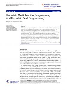
For different weights in (22) we obtained the results shown in Table 5. The optimal solution of the constrained problem is x1 = x2 = 0.3, xi = 0.05, i = 3, . . . , 10 with f (x) = (280.02, 240.8, 0.29, 4.5, 0.73) with utility U (y) = 87.8. It is remarkable that the same result was obtained by using the scalarization and utility function approaches. See the first row of Table 5 and the last row of Table 3, for example. The optimal solution of the unconstrained problem is x1 = 1 with f (x) = (432.89, 333.20, 0, 4, 1) with utility U (y) = 95.67. Note that this solution has also been calculated using the scalarization approach with the weights (4,5,6,7,8) or (1,1,1,1,1), for example (see Table 2). It is worth mentioning that using the conic scalarization method new and different efficient solutions have been obtained for the same set of weights (for different values of α). This means that the conic scalarization method provides several solutions for the given preferences and the resulting solution representing the decision maker’s preferences can be chosen among these. The optimal solution of the problem with optimal portfolio size is x1 = x2 = x3 = 0.3, x4 = 0.1, i.e. k = 4 with f (x) = (311.69, 291, 0, 4.1, 0.72) and utility U (y) = 89.41. Solving (22) for all feasible values of k we obtained the results shown in Table 6. Note that (22) is infeasible for k ≤ 3 since ri = 0.3. Figure 2 shows the decreasing utility values with increasing portfolio cardinality.
13
k 4 5 6 7 8 9 10 11 12 13 14 15 16 17 18 19 ≥ 20
Table 6: Optimal utility values for all feasible cardinalities. U (y) f1 f2 f3 f4 89.41 89.37 89.15 88.86 88.54 88.17 87.80 87.19 86.54 85.93 85.32 84.70 83.75 82.79 81.83 81.63 81.61
311.69 310.90 306.39 300.65 294.13 287.28 280.02 268.06 254.59 239.39 226.68 212.61 193.85 175.21 156.49 66.33 67.58
291.00 294.57 284.31 271.57 257.84 244.31 240.80 237.35 232.86 221.49 214.05 207.73 200.17 191.10 181.65 115.80 121.21
0.00 0.00 0.03 0.03 0.28 0.28 0.29 0.37 0.56 0.99 1.10 1.37 1.40 1.42 1.43 1.50 1.51
4.10 4.10 4.15 4.20 4.15 4.15 4.15 4.20 4.25 4.10 4.10 4.05 4.10 4.10 4.15 4.80 4.70
Maximal utility values for different portfolio size 90 88 86
U(y)84 82 80 78 76
4
8
12
16
20
24
28
32
36
40
Portfolio size (k)
Figure 2: The maximal utility of a portfolio decreases with increasing cardinality.
14
f5 0.72 0.71 0.69 0.70 0.71 0.73 0.73 0.72 0.71 0.67 0.67 0.66 0.65 0.64 0.64 0.62 0.62
5
Conclusion
In this paper we have explained two approaches to portfolio optimization. They differ in the sequence of elicitation of investor preference and optimization. While the multiobjective programming approach uses optimization first to find efficient solutions of a portfolio selection problem with multiple criteria for the investor to choose from, the multiattribute utility approach elicits preference information from the investor to construct a utility function which is subsequently optimized. While, under reasonable assumptions, both approaches will yield portfolios with the same utility, they do have quite unique challenges. The main challenge for the multiobjective programming approach is of a computational nature: Can (a representative subset of) the efficient solutions be computed, so that selecting a portfolio from this set guarantees a most preferred portfolio for the investor? If more than two criteria are used, computing all efficient solutions of a non-linear mixed integer programme such as (4) is not currently possible. There is some research on computing a set of representative efficient solutions, but this is restricted to linear programmes or integer linear programmes with two objectives. Such a set should reflect all the possible trade-offs between the criteria available in the set of efficient solutions, but be small enough to allow inspection by the investor. The advantage is clearly that the only assumption on the investor’s utility function is that the criteria represent all relevant attributes of a portfolio. For the multiattribute utility approach the major questions are of a methodological nature: Is an additive utility function justified? Is U sensitive to the choice of the reference set? What method for construction of the utility function and preference elicitation should be used? For example, for linear criteria functions fk it is clear that there are single assets for which the minimal and maximal values of fk (x) are attained, but for the variance this is not the case. Hence choosing the set of assets as reference set might give a false range of values in the construction of uk . The major advantage of the approach is that only one optimization is necessary to find the most preferred portfolio. In conclusion, the approach to solution of a portfolio optimization problem must be carefully considered by the investor.
References Arthur, L. and Ghandforoush, P. (1987). Subjectivity and portfolio optimization. In K. Lawrence, J. Guerard, and G. Reeves, editors, Advances in Mathematical Programming and Financial Planning, pages 171–186. JAI Press, Greenwich, CO. Ballestero, E. and Romero, C. (1996). Portfolio selection: A compromise programming solution. Journal of the Operational Research Society, 47, 1377–1386. Chang, T., Meade, N., Beasley, J., and Sharaiha, Y. (2000). Heuristics for cardinality constrained portfolio optimisation. Computers and Operations Research, 27, 1271–1302. Doumpos, M. and Zopounidis, C. (2002). Multicriteria Decision Aid Classification Methods, volume 73 of Applied Optimization. Kluwer Academic Publishers, Dordrecht. Ehrgott, M. (2005). Multicriteria Optimization. Springer-Verlag, Berlin, 2nd edition. Ehrgott, M. and Wiecek, M. (2005). Multiobjective programming. In J. Figueira, S. Greco, and M. Ehrgott, editors, Multicriteria Decision Analysis: State of the Art Surveys, pages 667–722. Kluwer Academic Publishers, Boston. Ehrgott, M., Klamroth, K., and Schwehm, C. (2004). An MCDM approach to portfolio optimization. European Journal of Operational Research, 155, 752–770. Gasimov, R. (2001). Characterization of the benson proper efficiency and scalarization in nonconvex vector optimization. In M. Koksalan, S. Zionts, and R. Steuer, editors, Multiple Criteria 15
Decision Making in the New Millenium, volume 507 of Lecture Notes in Economics and Mathematical Systems, pages 189–198. Geoffrion, A. (1968). Proper efficiency and the theory of vector maximization. Journal of Mathematical Analysis and Applications, 22, 618–630. Hallerbach, W. and Spronk, J. (1997). A multi-dimensional framework for portfolio management. In M. H. Karwan, J. Spronk, and J. Wallenius, editors, Essays in Decision Making. A Volume in Honour of Stanley Zionts, pages 275–293. Springer, Berlin. Keeney, R. L. and Raiffa, H. (1993). Decisions with Multiple Objectives: Preferences and Value Tradeoffs. Cambridge University Press. Konno, H. (1990). Piecewise linear risk function and portfolio optimization. Journal of the Operational Research Society of Japan, 33(2), 139–156. Markowitz, H. (1952). Portfolio selection. Journal of Finance, 7, 77–91. Markowitz, H. (1959). Portfolio Selection: Efficient Diversification of Investments. John Wiley & Sons, New York. Steuer, R. and Na, P. (2003). Multiple criteria decision making combined with finance: A categorized bibliographic study. European Journal of Operational Research, 150, 496–515. Steuer, R., Qi, Y., and Hirschberger, M. (2006). Suitable-portfolio investors, nondominated frontier sensitivity, the effect of multiple objectives on standard portfolio selection. Annals of Operations Research, In print.
16