THE JOURNAL OF CHEMICAL PHYSICS 128, 154718 共2008兲
Multiple histogram reweighting method for the surface tension calculation A. Ghoufi,1 F. Goujon,2 V. Lachet,1 and P. Malfreyt2,a兲 1
IFP, 1-4 Av. de Bois Préau, 92852 Rueil Malmaison Cedex, France Laboratoire de Thermodynamique des Solutions et des Polymères, UMR CNRS 6003, Université Blaise Pascal, 63177 Aubière Cedex, France
2
共Received 30 November 2007; accepted 11 March 2008; published online 21 April 2008兲 The multiple histogram reweighting method takes advantage of calculating ensemble averages over a range of thermodynamic conditions without performing a molecular simulation at each thermodynamic point. We show that this method can easily be extended to the calculation of the surface tension. We develop a new methodology called multiple histogram reweighting with slab decomposition based on the decomposition of the system into slabs along the direction normal to the interface. The surface tension is then calculated from local values of the chemical potential and of the configurational energy using Monte Carlo 共MC兲 simulations. We show that this methodology gives surface tension values in excellent agreement with experiments and with standard NVT MC simulations in the case of the liquid-vapor interface of carbon dioxide. © 2008 American Institute of Physics. 关DOI: 10.1063/1.2904460兴 I. INTRODUCTION
The calculation of the surface tension using molecular simulation can be performed using different methodologies. The most natural method consists in modeling two coexisting phases in physical contact in a liquid-slab arrangement. This methodology takes advantage of providing a molecular description of the interfacial region. However, it depends on the set up conditions 共truncation procedures,1–3 cutoff radius,1,4 long range corrections 共LRCs兲,2,4 and size of the simulation cell4,5兲. Other methodologies avoid the need to establish an interface. These approaches are based on the thermodynamic definition of the surface tension and express the surface tension from the contribution to the free energy due to the formation of the interface. Within the framework of free energy methods, the grand canonical transition matrix Monte Carlo6,7 共GC-TMMC兲 method determines the density dependence of the free energy of a fluid at a given temperature. When the GC-TMMC method is associated with the Binder approach,8 the surface tension is related to the free energy barrier between vapor and liquid phases, which is calculated from a GC-TMMC probability distribution.9–12 Within the Binder approach, the density dependence of the system can be explored with the aid of a histogram reweighting method.13,14 This approach has been successfully applied on Lennard-Jones6,9,15 共LJ兲, square well,10 n-alkanes,11 and LJ mixtures16 and is particularly attractive at relatively high temperatures along the liquid-vapor saturation line. A second general method based on the free energy of the system uses the ghost interface technique17 in conjunction with a modified Gibbs ensemble method for the simulation of adjacent coexisting phases. All these methods do not require the physical presence of the interface. The molecular simulations of the two-phase systems a兲
Author to whom correspondence should be addressed. Electronic mail:
[email protected].
0021-9606/2008/128共15兲/154718/12/$23.00
with the explicit presence of the interface allow us to calculate the surface tension and to describe the interfacial region at a molecular level. This leads to heterogeneous systems where a nonuniformity of the density number takes place along the direction normal to the interface. These two-phase simulations are challenging and special attention has to be paid on a certain number of factors: the time required to stabilize the formation of the interface, the validation of the thermodynamic equilibria 共thermal, mechanical, and chemical兲, the truncation effects involved in the calculation of the potential and corresponding force, and the procedures used for calculating the electrostatic contributions. The influence of these factors1–5,18 on the initial setup of the simulations has been extensively studied during these past years. A certain number of operational expressions have been established for the surface tension calculation. The most general working expression uses macroscopic normal and tangential pressures, which can be related to the derivative of the pair potential. The final form has been obtained by Kirkwood and Buff19–22 共KB兲 and gives a macroscopic scalar surface tension. In the case of a planar liquid-vapor interface lying in the x , y plane, the density gradient takes place in the z direction normal to the surface. The surface tension can be ⬁ expressed as 兰−⬁ (pN共z兲 − pT共z兲)dz, where pN共z兲 and pT共z兲 are local values of the normal and tangential components of the pressure tensor, respectively. Expressing the surface tension as a function of the local components of the pressure allows z us to use a local ␥共z兲 defined as 兰−⬁ (pN共z兲 − pT共z兲)dz. The use of ␥共z兲 is a key element to check the validity of the calculation concerning the stabilization of the interfaces, the independence between the two interfaces, and the constancy of ␥共z兲 in the bulk phases. We note that there are many ways of expressing the local components of the pressure, which depend on the contour joining two interacting molecules. Irving and Kirkwood23–26 共IK兲 used a straight line to join the two particles. This choice is the most natural and the one generally made. Nevertheless, the scalar value of surface tension is invariant to the choice of the pressure tensor. Until recently,
128, 154718-1
© 2008 American Institute of Physics
Downloaded 04 Jul 2008 to 194.214.132.32. Redistribution subject to AIP license or copyright; see http://jcp.aip.org/jcp/copyright.jsp
154718-2
J. Chem. Phys. 128, 154718 共2008兲
Ghoufi et al.
only the method of Irving and Kirkwood was designed to provide a profile of the surface tension. Both methods 共KB and IK兲 are based on the mechanical definition on the surface tension. Recently, the “test-area”27 共TA兲 method based on the perturbation formalism was proposed for the calculation of the surface tension. This method takes advantage of expressing the surface tension as a difference in energy between a reference state and a perturbed state characterized by an infinitesimal increase or decrease in the surface. However, the aspect of the local surface tension was missing within the Kirkwood–Buff expression and the TA method. This led us to establish the local expression of the surface tension calculated from the test-area approach3 and to propose the local version of the surface tension resulting from the virial route 共KBZ兲 in a recent work where KB refers to the KirkwoodBuff definition and Z indicates the direction of the gradient density.28 The surface tension can also be calculated from the amplitude of capillary waves23,29 at the liquid-vapor interface. The interface Hamiltonian30 can be linearized; it is found that the square of the interfacial thickness is related to the surface tension. It is then possible to calculate the surface tension from a series of simulations for systems of different interface sizes. This technique has been applied recently to the surface tensions of a polymer melt30 and of water.31 Additionally, the use of truncated potential requires adding LRCs to the thermodynamic properties and an inconsistent treatment of the LRCs to the surface tension can lead to conflicting results between the different methods. It is also essential to associate an appropriate expression of the tail correction with that of the intrinsic part of the surface tension. A certain number of expressions for calculating the LRC contributions of the surface tensions were developed.32–37 Some of them34–37 express the LRC contributions of the surface tension along the direction perpendicular to the interface. Our conclusions from a previous work3 showed that the different methods 共IK, TA, and KB兲 matched very well as long as appropriate LRC contributions were included in the calculation. We have also proposed the operational expression of the LRC profile3 of the surface tension within the TA approach. It is now well established that the LRCs of the surface tension can represent up to 30% of the total value for cutoff radii similar to those used for homogeneous systems. The methodology consisting in calculating the surface tension from a direct Monte Carlo 共MC兲 simulation with coexisting phases in physical contact is time consuming and a systematic study of the temperature dependence of these interfacial properties may represent a relatively cumbersome task. In order to improve the efficiency of the calculation, we aim at extending the histogram reweighting method, originally proposed to assess bulk properties, to the calculation of interfacial properties. The multiple histogram reweighting 共MHR兲 technique13,14 represents a powerful technique to extend the information obtained from MC simulations to different ther-
modynamic states. Additionally, this method increases the accuracy in the evaluation of the nonreweighted thermodynamic properties. Throughout this paper, we propose the development of the MHR methodology devoted to the surface tension using the IK definition. The methodology developed here can be used with other definitions of the surface tension as, for instance, the local definition of the TA method and the KBZ approach. We apply the developed methods to the calculation of the surface tension of the liquid-vapor interface of carbon dioxide. The paper is organized as follows. Section II contains the description of the IK definition for the surface tension calculation and the standard histogram reweighting methods. Section III presents the MHR method we have developed for a two-phase system. Section IV discusses the results of the surface tension as a function of the technique used, and Sec. V contains our conclusions. II. THEORETICAL BACKGROUND A. Surface tension calculation
In the case of a system baring two planar liquid-vapor surfaces lying in the x , y plane, where the heterogeneity takes place in the z axis normal to the interfaces, the surface tension can be calculated from the integration of the difference of the normal and tangential components of the pressure tensor of IK 共Refs. 19 and 23–26兲 across both interfaces according to
␥IK =
1 2
冕
+Lz/2
−Lz/2
dz„pN共z兲 − pT共z兲…,
共1兲
where pN共z兲 and pT共z兲 are the z components of the normal and tangential pressure tensors, respectively, calculated using Eq. 共2兲. This operational expression also provides a profile of the surface tension ␥IK共zk兲 defined as (pN共zk兲 − pT共zk兲)␦z. The total surface tension is then calculated via the half sum of the local surface tensions ␥IK共zk兲, p␣共zk兲 = 具共zk兲典kBTI −
1 A
⫻
冓
N−1 N
1 dU共rij兲 1 drij 兩zij兩
兺 兺 共rij兲␣共rij兲 rij i=1 j⬎i
冉 冊 冉 冊冔 zk − zi z j − zk zij zij
,
共2兲
where I is the unit tensor and T is the input temperature. ␣ and  represent x, y, or z directions. 共x兲 is the unit step function defined by 共x兲 = 0 when x ⬍ 0 and 共x兲 = 1 when x 艌 0. A is the surface area normal to the z axis. The distance zij between two molecular centers of mass is divided into Ns slabs of thickness ␦z. Following IK, the molecules i and j give a local contribution to the pressure tensor in a given slab if the line joining i and j crosses, starts, or finishes in the slab. Each slab has 1 / Ns of the total contribution from the i-j interaction. The normal component pN共zk兲 is equal to pzz共zk兲, whereas the tangential component is given by 21 (pxx共zk兲 + pyy共zk兲). We adopt the molecular definition of the pressure
Downloaded 04 Jul 2008 to 194.214.132.32. Redistribution subject to AIP license or copyright; see http://jcp.aip.org/jcp/copyright.jsp
154718-3
J. Chem. Phys. 128, 154718 共2008兲
Surface tension calculation
tensor using the center-of-mass definition. This operational expression also provides a profile of (pN共zk兲 − pT共zk兲)␦z. The corresponding LRCs are calculated by Eq. 共3兲 as proposed by Guo and Lu,35
␥IK,LRC共zk兲 = 共zk兲␦z 2
冕 冕 ⬁
r
dr
rc
− 共zk−i+1兲兴
−r
Ns
d⌬ z 兺 关共zk−i兲 共3兲
⌬z is the difference 共z − zk兲 and varies between −r and r. Ns is the number of slabs between zk and z. The first term is similar to that used in a homogeneous system except for the use of a number of density 共zk兲 depending on zk. The second term takes into account that each slab zk is surrounded with slabs of different local densities. In this relation, 共zk兲 is the local density of the zk slab and r represents the distance between the center of mass of two molecules. In Eq. 共3兲, ULJ,m is defined as Na Nb
ULJ,m共r兲 = 兺 兺 4⑀ab a=1 b=1
冋冉 冊 冉 冊 册 ab r
12
−
ab r
6
,
共4兲
where Na and Nb represent the number of force centers in molecules a and b, respectively.
ZNVT = 兺 exp„− E共兵␣其兲… = 兺 n共E兲exp共− E兲, 兵␣其
共5兲
E
where 兺兵␣其 represents the summation on the available states 共兵␣其兲 and n共E兲 is the density of states of energy E.  is the inverse temperature defined as 1 / kBT, where kB is the Boltzmann constant. At T⬘, the canonical partition function becomes ZNVT⬘ = 兺 n共E兲exp共− ⬘E兲
共6a兲
E
= 兺 n共E兲exp共− E兲exp„− 共⬘ − 兲E….
共6b兲
E
The MHR method takes advantage of collecting a series of histograms of the energy at nearby temperature overlap. We perform a series of R MC simulations in the canonical ensemble 共NVTi兲 corresponding to a different i inverse temperature. During these simulations we build a histogram hi共E兲 of the number of times that an energy E is observed, which is related to the density of states, n共E兲. The true distribution of no weighted energy is expressed as n共E兲exp共− iE兲 . 兺En共E兲exp共− iE兲
具X典⬘ = =
兺EX共E兲n共E兲exp共− ⬘E兲 兺En共E兲exp共− ⬘E兲
共7a兲
兺EX共E兲n共E兲exp„− 共⬘ − 兲E…exp共− E兲 . 兺En共E兲exp„− 共⬘ − 兲E…exp共− E兲
共7b兲
The counts of occurrence of energy H共E兲 can be determined up to a constant C共T兲 from the following expression:
共10兲
The reduced free energy f i is given by f i = −ln 兺En共E兲exp共−iE兲, thus exp共−f i兲 = 兺En共E兲exp共−iE兲. By using this expression, Eq. 共10兲 can be rewritten as Hi共E兲 =
n共E兲 . exp共iE − f i兲
共11兲
If we weight this distribution by the number of samples Ni in the simulation i, we obtain hi共E兲 hi共E兲 n共E兲 ⇒ n共E兲 = = exp共iE − f i兲, Ni exp共iE − f i兲 Ni 共12兲 where n共E兲 is calculated at a given inverse temperature i. If we calculate n共E兲 from different temperatures i, we combine R MC simulations and weight n共E兲 by pi共E兲 as R
n共E兲 = 兺 i
The average of the observable X in the canonical ensemble at T⬘ using the single histogram technique is given by
共9兲
C. MHR
13,38
The histogram reweighting method is a powerful technique that consists in extending the information extracted from a single MC simulation at an inverse temperature  to different temperatures. The canonical partition function ZNVT can be expressed in terms of density of states as
兺EX共E兲H共E兲exp„− 共⬘ − 兲E… . 兺EH共E兲exp„− 共⬘ − 兲E…
Single histogram reweighting gives reliable results only over a limited range of energies. If ⬘ differs too much from , the peak of the reweighted histogram will be shifted to the tails of the measured histogram, where the statistical uncertainty is high. In this case, it is recommended to use the MHR methodology outlined by Ferrenberg and Swendsen.14
Hi共E兲 =
B. Single histogram reweighting
共8兲
where the constant C共T兲 is only dependent on T. The average value of the X property using the single histogram method thus becomes 具X典⬘ =
i=1
dULJ,m 2 关r − 3共⌬z兲2兴. dr
H共E兲 = C共T兲n共E兲exp共− E兲,
pi共E兲hi共E兲 exp共iE − f i兲 Ni
R
with
兺i pi共E兲 = 1, 共13兲
where pi共E兲 indicates the relative weight of E by considering all simulations. Hi共E兲 = pi共E兲hi共E兲, where pi共E兲 is calculated by minimizing the error in n共E兲 (␦2n共E兲) by using the Lagrange multipliers. We define pi共E兲 as follows: pi共E兲 =
Ni exp„− 共iE − f i兲… 兺Rj N j exp„− 共 jE − f j兲…
.
共14兲
The improved estimate for the density of states becomes
Downloaded 04 Jul 2008 to 194.214.132.32. Redistribution subject to AIP license or copyright; see http://jcp.aip.org/jcp/copyright.jsp
154718-4
n共E兲 =
J. Chem. Phys. 128, 154718 共2008兲
Ghoufi et al.
兺Ri hi共E兲 兺Rj N j
exp„− 共 jE − f j兲…
共15兲
.
The calculation of the free energy f k at inverse temperature k is found self-consistently by iterating Eq. 共16兲. Let us recall that k denotes one of the reference systems and varies from 1 to R, where R is the total number of independent MC simulations.
We may express the expressions given in Eqs. 共16兲 and 共17兲 without building the histograms of energy and performing the sum over E first.39 By using this methodology, the calculation of f k can be done using Eqs. 共18a兲 and 共18b兲, and in a more operational expression, using Eq. 共18c兲 as follows: R i
exp共− f k兲 = 兺 n共E兲exp共− kE兲
R
E
=兺 E
兺Ri hi共E兲 兺Rj N j exp„− 共 jE − f j兲…
=兺 兺 i
R
兺EX共E兲n共E兲exp共− E兲 , 兺En共E兲exp共− E兲
共17兲
where 具X典 denotes the average of the X property at the  target inverse temperature.
具X典 =
具X典 =
R E 兺j Nj
exp共− kE兲. 共16兲
Once the value of f k is obtained, we can calculate n共E兲 and estimate the average of the observable X at the inverse temperature  according to 具X典 =
hi共E兲exp共− kE兲 R E 兺 j N j exp„− 共 jE − f j兲…
exp共− f k兲 = 兺 兺
=兺 兺 i
兺Ri 兺␣Xi␣共兺Rj N j exp共− „共 j − 兲Ei␣ − f j…兲兲−1
exp共− „共 j − k兲E − f j…兲 1 exp共− „共 j − k兲Ei␣ − f j…兲
共18b兲
, 共18c兲
where ␣ in Eq. 共18c兲 represents the ␣ configuration in the i MC calculation. Whereas the average of the observable X requires in Eq. 共19兲 the calculation of the histograms of E, the new operational expression of Eq. 共20兲 uses the fact that the reweighted average of X can be performed without histograms as follows:
兺EX共E兲共兺Ri hi共E兲兲共兺Rj N j exp„− 共 jE − f j兲…兲−1 exp共− E兲 兺E共兺Ri hi共E兲兲共兺Rj N j exp„− 共 jE − f j兲…兲−1 exp共− E兲
R ␣ 兺j Nj
hi共E兲
共18a兲
,
共19兲
.
共20兲
III. HISTOGRAM REWEIGHTING METHODOLOGY FOR A TWO-PHASE SYSTEM
factors contributing to the efficiency of the MHR methodology. To evaluate the importance of fluctuations, we define the following coefficient: r = ␦E / 具E典. In the case of the liquidvapor interface of carbon dioxide at 238 K, r is equal to 2.3⫻ 10−2 for the total simulation box, whereas it is equal to 0.6 and 3.8 for each slab of the liquid and vapor phases, respectively. As concerns the determination of the coexistence curves of tiophene using grand canonical MC combined with histogram reweighting methods,40 r is equal to 0.7 and 2.4 in the liquid and vapor phases, respectively. We show that it is possible to converge to the same values of r when the system is decomposed into slabs. In what follows, we extend the MHR methodology to systems with slab decompositions 共MHRS兲. Let us recall that the MC simulation is carried out in the constant-NVT ensemble. The simulation box is divided into Ns slabs of width ␦z and volume Vs = LxLy␦z. The total number of molecules N is constant, whereas the number of molecules Nzk in each slab fluctuates within the simulation. This is equivalent to fixing the chemical potential zk of the considered species at each zk position. The grand canonical partition function of the slab zk can be written as
兺Ri 兺␣共兺Rj N j exp共− „共 j − 兲Ei␣ − f j…兲兲−1
A. Multiple histogram reweighting for each slab „MHRS…
In the case of the simulation of a planar liquid-vapor surface lying in the x, y plane where a heterogeneity takes place in the z axis normal to the interface, we expect a dependence of the thermodynamic properties only in this z direction. This nonuniformity of the density imposes accounting for some local definitions of thermodynamic properties 共pressure and energy density兲. We have also established in previous papers the uniformity of the local chemical potential, temperature, and pressure components for the liquidvapor interfaces of n-alkanes. It is then very appropriate to develop a local version of the MHR method for the surface tension calculation. Additionally, when we focus on the fluctuations of the total energy of the simulation box during a MC simulation, we observe that they are very weak, and MC simulations of a two-phase system require very large systems to stabilize the interface. The two criteria, large fluctuations of the energy and a relatively small system, are important
Downloaded 04 Jul 2008 to 194.214.132.32. Redistribution subject to AIP license or copyright; see http://jcp.aip.org/jcp/copyright.jsp
154718-5
J. Chem. Phys. 128, 154718 共2008兲
Surface tension calculation
⌶共zk,Vzk, 兲 = 兺 兺 ⍀共Nzk,Vzk, 兲exp„− 共Uzk − zkNzk兲…, Nz Uz k k
k
k
共22兲
k
共21兲 where zk is the chemical potential of the slab at zk,  is the inverse temperature, Uzk is the energy of the slab at zk, and ⍀共Nzk , Vzk , 兲 is the canonical density of states. Writing Eq. 共21兲 amounts to defining a local grand potential partition function. This leads to assuming the absence of correlations between neighboring slabs. In this case, all the slabs can be treated independently. The partition function of the system in the NVT ensemble can be expressed as
R
exp共− f l,zk兲 = 兺 兺 i
兿z ⌶共z ,Vzk,Tz 兲 ⯝ 兺N 关exp共N兲Q共N,V, 兲兴.
␣
冉兺
Assuming the existence of this local partition function and Ns satisfying the following criteria, N = 兺i=1 Nzi and 兰VdzkUzk = U, it is then possible to establish the expression given in Eq. 共22兲. The different steps leading to the final expression of Eq. 共22兲 are given in Appendix A. The existence of the local partition function allows the application of the MHR methodology to each slab. If we follow the same procedure as that used for the MHR in the canonical ensemble, we obtain the expressions of Eqs. 共23兲 and 共24兲. An accurate demonstration has been performed by Pérez-Pellitero et al.39 and Shi and Johnson41 in the VT ensemble.
R j
N j exp共− „共 j − l兲Ei␣,zk − ni␣,zk共 j j,zk − ll,zk兲 − f j,zk…兲
冊
−1
,
共23兲
where l denotes the reference systems. 具X典,zk =
兺Ri 兺␣Xi␣,zk共兺Rj N j exp共− „共 j − 兲Ei␣,zk − ni␣,zk共 j j,zk − ,zk兲 − f j,zk…兲兲−1 兺Ri 兺␣共兺Rj N j exp共− „共 j − 兲Ei␣,zk − ni␣,zk共 j j,zk − ,zk兲 − f j,zk…兲兲−1
where l varies from 1 to R, and ,zk is the total chemical potential of the slab k at the inverse target temperature . Ei␣,zk is the energy of the slab at the position zk at the inverse temperature i for the ␣ configuration and is defined as N
N
N
N
a b 1 Ezk = 兺 兺 兺 兺 Hk共zi兲U共riajb兲, 2 i=1 j⫽i a b
共25兲
where U共riajb兲 is the sum of the 6-12 LJ and electrostatic energy contributions in the slab k, and Hk共zi兲 is a top-hat function with functional values of
␦z
Hk共zi兲 = 1
for zk −
Hk共zi兲 = 0
otherwise.
2
⬍ zi ⬍ zk +
␦z 2
, 共26兲
We adopt the definition of Ladd and Woodcock42 and choose to assign in the slab centered on zk two energy contributions: one contribution due to the energy between the molecules
具典,zk =
共24兲
,
within the slab and a second contribution due to the energy of the molecules within the slab with those outside the slab. By using this definition, we respect the following condition:
冕
V
共27兲
dzkUzk = E,
where E is the total configurational energy of the simulation box and V its volume. In Eqs. 共23兲 and 共24兲, the difficulty lies in the calculation of the local chemical potential 共,zk兲 at the  inverse temperature. To avoid additional simulations, we use a self-consistency approach consisting in calculating the chemical potential at the inverse temperature . We apply an iterative process to resolve Eq. 共28兲. Once the value of 共,zk兲 is obtained, we repeat a new iterative process for the calculation of the observable property as in Eq. 共24兲. To summarize the different steps, the calculation of f l,zk 关Eq. 共23兲兴 is first carried out, then we calculate 具典,zk 关Eq. 共28兲兴, and we finish with 具X典,zk using Eq. 共24兲 as follows:
兺Ri 兺␣i␣,zk共兺Rj N j exp共− „共 j − 兲Ei␣,zk − ni␣,zk共 j j,zk − 具典,zk兲 − f j,zk…兲兲−1 兺Ri 兺␣共兺Rj N j exp共− „共 j − 兲Ei␣,zk − ni␣,zk共 j j,zk − 具典,zk兲 − f j,zk…兲兲−1
,
共28兲
where n␣,zk is the number of molecules in the slab zk for the ␣ configuration. Ei␣,zk represents the total energy of the slab zk calculated from the sum of the intrinsic contribution given by Eq. 共25兲 and of the LRC part given by the following expression: 共1兲 共2兲 共zk兲 + ULRC 共zk兲 = 22共zk兲Vs ULRC共zk兲 = ULRC
冕
⬁
rc
dr r2ULJ,m共r兲 + 共zk兲Vs
冕 冕 ⬁
r
dr
rc
d⌬ z关共z兲 − 共zk兲兴rULJ,m共r兲.
共29兲
−r
Downloaded 04 Jul 2008 to 194.214.132.32. Redistribution subject to AIP license or copyright; see http://jcp.aip.org/jcp/copyright.jsp
154718-6
J. Chem. Phys. 128, 154718 共2008兲
Ghoufi et al.
B. Calculation of a local chemical potential
The calculation of the chemical potential allows us to check the local chemical equilibrium of a system where a nonuniformity of the density takes place along a specific direction. In the case of the constancy of the chemical potential throughout the z direction of the heterogeneity, we may use the decomposition of the system into open subsystems with constant local chemical potential.3 Different techniques have been used for the calculation of the chemical potential. Among them, the original test particle insertion method of Widom43 has been widely applied for the calculation of the chemical potential in homogeneous systems. This method consists in inserting a ghost particle randomly into a simulation box of N molecules and calculating the interaction energy of its ghost particle with the N molecules. As concerns the calculation of the chemical potential in heterogeneous systems, Widom44 has changed the original version in such a way as to account for the dependence of on the local density zk. However, in the case of systems involving both electrostatic interactions and high density, the test particle insertion can no longer be applied. One alternative consists in making the insertion easier by decomposing the move into two steps: the insertion of a LJ center and the calculation of the electrostatic contribution resulting from a perturbation process. This method gives accurate results for homogeneous systems, but the extension of this methodology for heterogeneous systems is time consuming due to the need for obtaining a profile of the chemical potential along the axis where a nonuniformity exists. Instead, we perform an insertion scheme with biased positions and orientations45–47 for the calculation of the local chemical potential in a heterogeneous system. This method involves in a first step the selection of an appropriate location for the center of mass of the considered inserted molecule by n test insertions of a LJ particle, whose properties depend on the type of molecule to be inserted. In a second step, m orientations are tested in the selected location, with the full potential defined as the sum of the LJ and electrostatic energy contributions. Within this formalism, the chemical potential is then given by
= − kT ln
冓
with
冉 冉兺
冔
共30兲
− ⌬ULJ,zk兲…
冔
共32兲
, z Vz Tz k k k
冉 冉兺
冊
k
WLJ,zk =
1 兺 exp„− 共⌬ULJ,i,zk兲… , k i=1
Wor,zk =
共33兲
冊
m
1 exp„− 共⌬U j,zk兲… , m j=1
where 具¯典z Vz  indicates the average ensemble in the grand k k canonical ensemble. In Eqs. 共32兲 and 共33兲, the definition of the different properties are similar to that given in Eqs. 共30兲 and 共31兲 except for the fact that these properties are calculated within each slab located at zk. We make the assumption that the average of the ratio 具共zk兲 / WLJ,zkWor,zk exp(−共⌬Ucor,zk − ⌬ULJ,zk兲)典 can be replaced by the ratio of the two averages 具共zk兲典 / 具WLJ,zkWor,zk exp(−共⌬Ucor,zk − ⌬ULJ,zk兲)典. This approximation has been validated in a previous study,3 where we checked that the difference between these averages is 10−5 unit. The resulting local chemical potential along the z direction can be calculated via the following expression:
共zk兲 = kT ln 具共zk兲⌳3典z Vz Tz k
k
k
k
k
= id共zk兲 + ex共zk兲,
共34兲
where id共zk兲 + ex共zk兲 are the local ideal and excess contributions of the chemical potential. To take into account the LRC of the local chemical potential, we use the local expressions proposed by Guo and Lu,35
冊
冊
1 V zk WLJ,zkWor,zk exp„− 共⌬Ucor,zk ⌳ 3 N zk + 1
k
1 WLJ = 兺 exp„− 共⌬ULJ,i兲… , k i=1 m
冓
− ⌬ULJ,zk兲…典z Vz Tz
NVT
k
共zk兲 = − kT ln
− kT ln 具WLJ,zkWor,zk exp„− 共⌬Ucor,zk
1 V WLJWor exp„− 共⌬Ucor ⌳3 N + 1
− ⌬ULJ兲…
⌬ULJ is the energy variation corresponding to the test insertion of the LJ particle in the selected location and ⌬Ucor represents the variation of the LRCs corresponding to the insertion of the molecule. ⌬U in Eq. 共31兲 denotes the sum of the LJ and electrostatic energy contributions. In the case of a nonuniformity of the density along the z direction, we extend the expressions of Eqs. 共30兲 and 共31兲 to the following expressions:
共31兲
1 Wor = exp„− 共⌬U j兲… , m j=1 where ⌳ is the de Broglie thermal wavelength. 具¯典NVT indicates the canonical ensemble average, V is the volume of the system, and N is the total number of particles. WLJ and Wor are the Rosenbluth factors associated with the selection of the test location and of the various orientations, respectively.
LRC共zk兲 = 4共zk兲
冕
⬁
dr r2ULJ,m共r兲
rc
+ 2
冕 冕 ⬁
rc
Ns/2
r
dr
−r
d⌬ z
兺
i=−Ns/2
− 共zk−i+1兲兴rULJ,m共r兲.
关共zk−i兲 共35兲
Finally, the total chemical potential is expressed as the sum of id共zk兲, ex共zk兲, and LRC共zk兲.
Downloaded 04 Jul 2008 to 194.214.132.32. Redistribution subject to AIP license or copyright; see http://jcp.aip.org/jcp/copyright.jsp
154718-7
J. Chem. Phys. 128, 154718 共2008兲
Surface tension calculation
TABLE I. CO2 force field 共Ref. 49兲 and description of the system. CO2 potential parameters
共Å兲
⑀ 共K兲
Charge 共e兲
C 2.757 O 3.033 C v O distance 共Å兲 O v C v O angle 共deg兲
28.129 80.507
+0.6512 −0.3256 1.149 180
MC parameters Lx = Ly 共Å兲 Lz 共Å兲 共Å−1兲 hxmax = hmax y hzmax 共Å−1兲
25.4 150.8 9 41
IV. RESULTS AND DISCUSSIONS
We apply the different techniques presented here for the calculation of the surface tension of the liquid-vapor interface of carbon dioxide. The simulation box is a rectangular parallelepipedic box of dimensions LxLyLz 共Lx = Ly兲 with 共N = 512兲 CO2 molecules. The details of the geometry of the system are given in Table I. The periodic boundary conditions are applied in the three directions. MC simulations are performed in the NVT ensemble. Each cycle consists of N randomly selected moves with fixed probabilities. Two types of MC moves are performed with probabilities of 0.5 each: the translation of the center of mass of a random molecule and the rotation of a randomly selected molecule around its center of mass. The initial configuration has been built by placing N molecules on the nodes of a fcc lattice included in a cubic box with random orientations. MC simulations in the NpT ensemble have been performed first on this bulk monophasic fluid configuration. The dimension of the resulting box has been increased along the z axis by placing two empty cells on both sides of the bulk liquid box. A typical MC run consists of 200 000 cycles for equilibration and 200 000 cycles for the production phase. The thermodynamic properties are calculated every ten cycles, leading to the storage of 20 000 configurations. The statistical errors for these properties are estimated using the jackknife method.48 This method uses four superblocks which are formed by combining three blocks of 5000 configurations. As the geometry of the system shows a heterogeneity along the axis normal to the interface 共z axis兲, we expect thus a dependence of the thermodynamic properties only in this direction. We have therefore calculated the local thermodynamic properties and their LRC as a function of zk by splitting the cell into slabs of width ␦z. The CO2 molecule is described using the rigid version of the Harris–Yung potential49 with three LJ centers and three electrostatic charges 共see Table I兲. The carbon-oxygen bond lengths are fixed and equal to 1.149 Å and the carbon dioxide molecule has a fixed OCO angle of 180°. The intermolecular interactions are modeled using the 6–12 LJ potential. The unlike interatomic interactions are calculated using the Lorentz–Berthelot combining rules, i.e., a geometric combining rule for the energy and an arithmetic combining rule for
the atomic size. We use a relatively small cutoff of 12 Å to make the two-phase simulations in line with those carried out in the Gibbs ensemble Monte Carlo 共GEMC兲 method.50–52 In this case, the use of the LRCs to be added to the interfacial properties is meaningful. We have also shown4 that the value of the surface tension calculated from MC simulations becomes independent of the cutoff radius once the LRCs are included. For systems with electrostatic interactions calcumax lated using the Ewald technique,53,54 we take hmax x = hy = 9 max and hz = 41 with respect to both the ratio of the box dimensions and the convergence of the reciprocal space contribution of the surface tension. The calculation of the surface tension from the simulation of two-phase systems can be affected by the use of both periodic boundary conditions and small surface areas.5,55 These recent works established an oscillatory function of the intrinsic part of the surface tension of LJ fluids for small surface areas and a constant value of the surface tension with larger surface areas. Beyond an interfacial area of 共7 ⫻ 72兲, where is the diameter of the LJ particle, we observe that the maximum variation in the intrinsic part of the surface tension does not exceed 15% of the constant value of ␥. The interfacial area used in this work approximately corresponds to the value of 共7 ⫻ 72兲. Let us recall that we must maintain an objective of computational efficiency for the two-phase simulation with respect to the simulation carried out with the GEMC methods.50 As a result, we aim to find a compromise between the system size and the CPU time. Then we evaluate the impact of the box dimensions on the calculation of the surface tension by keeping the surface area constant and changing the Lz dimension, and vice versa. Direct Monte Carlo simulations were then performed for N = 512, 768, and 1024 system sizes for the liquid-vapor interface of CO2 at T = 238 K. The different contributions of the surface tensions are given in Table II for the KB, IK, TA, and KBZ approaches. We do not observe a trend of the surface tension over this range of system sizes. The results show that the total surface tension is a little dependent on the system size for the systems studied here due to the fact that the changes in the surface tension are within the fluctuations estimated using the variation in the block averages. Additionally, the variations in the surface tension are comparable to those induced by the calculation of ␥ using different definitions. The magnitude of the fluctuations of the surface tension can be attributed to the fact that we are simulating molecular systems interacting through dispersion-repulsion and electrostatic interactions in contrast to those obtained in the simulation of LJ fluids. These fluctuations are of the same order of magnitude as those induced by the dependence of the surface tension with the surface area beyond an area of 共7 ⫻ 72兲. The fact that the surface tension remains unchanged within the statistical fluctuations when increasing the system size has already been observed for the calculation of the surface tension of water.18 It was also established by Guo and Lu35 that taking into account the LRC’s contributions to the configurational energy in the Metropolis scheme allows us to obtain reliable surface tensions with a smaller total
Downloaded 04 Jul 2008 to 194.214.132.32. Redistribution subject to AIP license or copyright; see http://jcp.aip.org/jcp/copyright.jsp
154718-8
J. Chem. Phys. 128, 154718 共2008兲
Ghoufi et al.
TABLE II. Surface tension values 共mN m−1兲 of carbon dioxide at T = 238 K calculated from MC simulations using different box dimensions and different numbers of molecules. The LRC contribution and the total surface tension are given for each method. The subscripts give the accuracy of the last decimal共s兲, i.e., 11.810 means 11.8⫾ 1.0. The experimental surface tensions 共Ref. 57兲 共␥expt.兲 are reported for comparison.
␥KB
␥IK
T 共K兲
␥LRC
␥TOT
␥LRC
238
3.12
11.810
238
3.02
238
238
␥TA ␥TOT
␥TOT
␥LRC
␥TOT
␥expt.
2.55
N = 512, Lx = Ly = 25.4 Å, Lz = 150.8 Å 11.510 1.85 11.710
2.13
11.010
12.0
11.910
2.15
N = 768, Lx = Ly = 32.4 Å, Lz = 150.8 Å 11.810 2.35 12.610
2.03
11.910
12.0
3.52
12.110
2.25
N = 1024, Lx = Ly = 25.4 Å, Lz = 200.8 Å 11.510 2.15 11.810
1.93
11.910
12.0
2.91
11.910
2.63
N = 1024, Lx = Ly = 32.4 Å, Lz = 200.8 Å 11.210 1.74 11.810
2.03
11.210
12.0
number of molecules. We have also underlined this point in the case of a previous work4 dealing with the calculation of surface tensions of n-alkanes. Before paying further attention to the MHR results, we have tested the single histogram reweighting formalism on the calculation of the surface tension of CO2 at 248 K from the reference temperature of 238 K. From the surface tension calculated by MC simulation using the IK definition at 238 K 共␥IK = 11.5 mN−1兲, we find that the single histogram reweighting method gives ␥IK = 12.5 mN−1 at 248 K. We observe that this methodology is not appropriate and leads to a value of surface tension that increases as the temperature increases. The surface tensions at 248 K resulting from MC simulation and from experimental measurements are equal to 10.8 and 9.7 mN−1, respectively. In the cases of the MHR and MHRS methods, we have tested two types of calculations: one involving three reference temperatures 共238, 248, and 298 K兲 and a second using seven reference temperatures 共238, 248, 258, 268, 278, 288, and 298 K兲. Figure 1 shows the calculated surface tensions using the MHR technique with three and seven reference temperatures. The experimental and calculated surface tensions at seven reference temperatures are reported in Table III and presented in Fig. 1 for comparison. We observe that the use of three reference temperatures does not lead to a good reproduction of the surface tensions in the range of temperatures studied. Calculating the surface tension with seven reference temperatures decreases the discrepancy but does not allow a good prediction of ␥ for temperatures lower than the lowest reference temperature, i.e., 238 K, because this zone is outside the temperature range covered by the reference temperatures. No extrapolation attempts have been performed in the high temperature region because calculations are restricted to temperatures below the critical temperature of CO2, which is 304 K. Figure 1 shows the high sensitivity of the MHR technique to the convergence quality of the reference MC simulations. A slight overestimate or underestimate of a single point can strongly affect the global trend of the surface tension evolution with temperature. The challenge of this work is to combine a relatively small number of reference temperatures and a good prediction of the surface tensions. To do so, we apply our MHRS methodol-
␥LRC
␥KBZ
ogy, which consists in applying the MHR technique to local surface tensions. Such calculations are based on the calculation of the local chemical potential. Figure 2共a兲 shows the profile of the total chemical potential calculated from the sum of the contributions given in Eqs. 共34兲 and 共35兲 at 248 K. As expected for a system at chemical equilibrium, we observe that the total chemical potential is constant throughout the z direction. We have already shown that the total chemical potential is independent of zk in the case of a liquid-vapor interface of n-alkanes.3 In
FIG. 1. 共Color online兲 共a兲 Surface tension values of the liquid vapor of CO2 calculated from MC simulations and experiments. The calculated points constitute the sets of three and seven reference temperatures. 共b兲 Surface tensions of CO2 calculated from the MHR technique with three and seven reference temperatures as indicated in the legend.
Downloaded 04 Jul 2008 to 194.214.132.32. Redistribution subject to AIP license or copyright; see http://jcp.aip.org/jcp/copyright.jsp
154718-9
J. Chem. Phys. 128, 154718 共2008兲
Surface tension calculation
TABLE III. LRCs and intrinsic and total contributions of the surface tension 共mN m−1兲 calculated from MC simulations. Experimental values 共Ref. 57兲 are given for comparison. The subscript indicates the accuracy of the last decimal共s兲. The number 11.510 means 11.5⫾ 1.0. T 共K兲
␥IK,LRCa
␥IKb
␥Total
␥Expt.
238 248 258 268 278 288 298
2.55 2.25 1.95 1.55 1.15 0.85 0.45
9.010 8.610 6.310 3.810 2.45 1.86 0.31
11.510 10.810 8.210 5.310 3.55 2.66 0.75
12.0 9.7 7.6 5.5 3.6 2.0 0.6
Equation 共1兲. Equation 共3兲.
a
b
the case of a carbon dioxide liquid-vapor interface, let us recall that the calculation requires more sophisticated algorithms due to the insertion of a molecule requiring the calculation of electrostatic energy contributions. We also checked that the total chemical potential recalculated from Eq. 共28兲 by using the MHRS methodology respects the chemical equilibrium in the two-phase system. In the calculation of 具典,zk from Eq. 共28兲, we need to save j,zk, which represents the chemical potential of a configuration j at a slab k. The calculation of in Eq. 共34兲 exhibits the presence of a logarithm of the average of an exponential term. It means that the operational expression of of Eq. 共34兲 cannot be decomposed into instantaneous values. We decided to apply the MHRS methodology on the term WLJ,zkWor,zk exp(−共⌬Ucor,zk − ⌬ULJ,zk兲) and to use this term instead of in Eq. 共28兲. Figure 2共b兲 displays the profile of the excess part of the chemical potential at 248 K. From this curve, it is then possible to extract the excess chemical potential of the vapor and liquid phases by fitting the profile with a hyperbolic tangent function defined as
冉 冊
1 l 1 l z − zo v v ex共zk兲 = 共ex + ex 兲 − 共ex − ex 兲tanh , 共36兲 2 2 d l v and ex are the excess chemical potentials of the where ex liquid and vapor phases, zo is the position of the Gibbs dividing surface, and d is an approximate measure of the thickness of the interface. We presented in Fig. 2共c兲 the ⌬ex l v = ex − ex contribution calculated from Eq. 共36兲. We compared the resulting values to the expression derived by BenNaim et al.56 关⌬ex = −kBT ln共l / v兲兴, where l and v are the experimental coexisting densities of the liquid and vapor phases, respectively. We observed that the calculated ⌬ex term matches quite well with the experimental value, indicating the correctness of the extension of the bias insertion scheme to a slab version in a two-phase system. Additionally, we presented on the right axis of Fig. 2共c兲 the total chemical potential calculated from both the GEMC simulations of homogeneous liquid and vapor phases using Eq. 共30兲 and the direct MC simulations of the corresponding two-phase system using Eq.共34兲. We checked that the calculated chemical potential are similar within the error bars. We also checked that the calculation of the local chemical potential using the
FIG. 2. 共Color online兲 共a兲 Total chemical potential profiles of the CO2 liquid-vapor interface at 248 K calculated from the sum of the contributions of Eqs. 共34兲 and 共35兲 and from the MHRS procedure with Eq. 共28兲. 共b兲 Excess chemical potential profiles with parts calculated from the Rosenbluth scheme 关Eq. 共32兲兴 and from the fit using Eq. 共36兲. 共c兲 Total chemical potential values 共right axis兲 calculated from GEMC simulations using Eq. 共30兲 共䉱兲 and from the two-phase simulation using Eqs. 共34兲 and 共35兲 共⽧兲. The difference of excess chemical potential values 共left axis兲 calculated using Eq. 共36兲 共䊊兲 and using ⌬ex = −kBT ln共l / v兲 共solid line兲, where l and v are the experimental coexisting densities 共Ref. 57兲 of the liquid and vapor phases, respectively.
configurational-bias scheme leads to the constancy of the chemical potential at each zk and provides values in agreement with the corresponding values57 derived from experimental densities. We now focus on the prediction of the surface tension using the MHRS technique. Figure 3 shows the surface tension values calculated using the methodology developed in this paper using either three or seven reference temperatures. Interestingly, we ob-
Downloaded 04 Jul 2008 to 194.214.132.32. Redistribution subject to AIP license or copyright; see http://jcp.aip.org/jcp/copyright.jsp
154718-10
J. Chem. Phys. 128, 154718 共2008兲
Ghoufi et al.
APPENDIX A: RELATIONSHIP BETWEEN ⌶,V, AND 兿z⌶„zk , Vzk , …
The local partition function in the grand canonical ensemble can be expressed as ⌶共zk,Vzk,Tzk兲 = 兺 exp共Nzk兲Q共Nzk,Vzk,Tzk兲 N
= 兺 兺 exp共zkNzk兲exp共− Ul zk兲. N
N
l
共A1兲 The product for zk is equal to FIG. 3. 共Color online兲 Surface tension values of the liquid vapor of CO2 calculated with the MHRS methodology using different procedures as indicated in the legend.
serve that the MHRS methodology gives surface tensions in line with the experimental values even in the case of three reference temperatures. We conclude that the adopted methodology 共MHRS兲, which consists in calculating local surface tensions from local configurational energy and local chemical potential, is efficient even in the case of using a relatively small number of reference temperatures. It was a prerequisite to make the MHRS methodology an efficient and powerful technique for the surface tension calculation. When the number of reference points is fixed to 7, we observed that the MHRS significantly improves the calculated values, leading to surface tensions in excellent agreement with the experimental ones.57
兿z ⌶共z ,Vz ,Tz 兲 k
k
= 兿 兺 exp共zkNzk兲Q共Nzk,Vzk,Tzk兲
共A2a兲
zk Nz k
=
冋兺 冋兺 Nz
exp共z1Nz1兲Q共Nz1,Vz1,Tz1兲
1
Nz
册
exp共z2Nz2兲Q共Nz2,Vz2,Tz2兲
⫻
2
册
共A2b兲
=关exp共z1Nz1 兲Q共Nz1,Vz1,Tz1兲 1
+ exp共z1Nz2 兲Q共Nz1,Vz1,Tz1兲兴 1
⫻ 关exp共z2Nz1 兲Q共Nz2,Vz2,Tz2兲 2
+ V. CONCLUSIONS
We have extended the standard MHR method to a new version that allows us to calculate local surface tensions from local configurational energies and local chemical potentials. The different steps essential to the use of the MHRS method have been discussed and the operational expressions of the local chemical potential, of the local configurational energies, and of their LRCs have been presented. The results of this new technique, called MHRS in this paper, are very promising. The calculated surface tensions of the liquidvapor interface of carbon dioxide are found to be in excellent agreement with the experimental ones even in the case of a small number of reference temperatures. We have also checked the chemical equilibrium of the system by presenting the profile of the total chemical potential calculated from the configurational-bias scheme. The MHRS methodology can be applied to different approaches for the calculation of the surface tension. However, these approaches must allow a local definition of the surface tension as, for example, the TA 共Ref. 3兲 and the KBZ 共Ref. 28兲 methods.
k
k
exp共z2Nz2 兲Q共Nz2,Vz2,Tz2兲兴 2
⫻ ¯.
共A2c兲
In this expression, the superscripts 1 and 2 indicate the various sampled states, whereas the subscripts denote the number of the slab. When we consider the terms satisfying the constraints relative to the total energy and to the total number Ns of molecules 共N = 兺i=1 Nzi and 兰VdzkUzk = U兲 and the fact that the local chemical potential and the local temperature are constant at each zk and equal to and T, respectively, we obtain
兿z ⌶共z ,Vzk,Tz 兲 = 兺N k
k
k
冋
册
exp共N兲 兿 Q共Nzk,Vzk,Tzk兲 . zk
共A3兲 By following the same reasoning and using the same constraints, we can write 兿zkQ共Nzk , Vk , Tzk兲 ⯝ Q共N , V , T兲. This allows us to write the following expressions:
兿z ⌶共z ,Vzk,Tz 兲 ⯝ 兺N 关exp共N兲Q共N,V,T兲兴,
共A4兲
兿z ⌶共z ,Vzk,Tz 兲 ⯝ ⌶共,V,T兲.
共A5兲
k
k
k
k
k
k
ACKNOWLEDGMENTS
One of the authors 共A.G.兲 is grateful to Carlos Draghi Nieto and Javier Pérez-Pellitero for stimulating discussions.
Equation 共A5兲 allows us to assume the existence of a local partition function. The relationship between ␥,V,T and ␥N,V,T is established in Appendix B.
Downloaded 04 Jul 2008 to 194.214.132.32. Redistribution subject to AIP license or copyright; see http://jcp.aip.org/jcp/copyright.jsp
154718-11
J. Chem. Phys. 128, 154718 共2008兲
Surface tension calculation
APPENDIX B: TRANSFORMATION OF ␥,V,T TO ␥N,V,T
Q共Nref,V,T兲 = ⌶共,V,T兲共Nref兲exp„− 共Nref兲…
共B1a兲
The demonstration of the relationship between ⌶共 , V , T兲, NrefQ共 , V , T兲, and Q共Nref , V , T兲 has been carried out by Gloor et al.27 Here Nref is the number of particles in the case of a restricted grand canonical partition function ⌶共 , V , T兲共Nref兲 for systems containing just Nref particles. The partition function in canonical ensemble for Nref is equal to
=⌶共,V,T兲exp„− 共Nref兲…P共Nref兲,
共B1b兲
兿z ⌶共,Vzk,T兲 ⯝ ⌶共,V,T兲 ⯝ k
where ⌶共 , V , T兲 is the grand canonical partition function and P共Nref兲 is the probability density of finding exactly Nref in any element of configurational space drNref. By using this definition, we can express the product of the local partition functions of Eq. 共A5兲 as
⌶共,V,T兲共Nref兲 Q共Nref,V,T兲exp„共Nref兲… ⯝ . P共Nref兲 P共Nref兲
共B2兲
We now consider the calculation of the macroscopic surface tension as a perturbation of the free energy with respect to the surface. ␥ = 共F / A兲VT. If we use a finite difference to calculate ␥, the free energy can be expressed by a partition function according to a statistical mechanics definition,
兺z ␥ k
zk,Vzk,T
=−
⌶共,Vzk,T,A兲 兿zk⌶共,Vzk,T,A兲 kT kT ln =− ln 兿 2⌬A 兿zk⌶共,Vzk,T,A + ⌬A兲 2⌬A zk ⌶共,Vzk,T,A + ⌬A兲
冤
共B3a兲
冥
Q共Nref,V,T,A兲exp„共Nref兲… kT P共Nref,A兲 ⯝− . ln 2⌬A Q共Nref,V,T,A + ⌬A兲exp„共Nref兲… P共Nref,A+⌬A兲
The transformation for the change in the surface area conserves the volume of each slab. We suppose that the chemical equilibrium is maintained between the reference and the perturbed states and that the probabilities of finding the system in the configuration spaces drNref and dr⬘Nref are very close, where the r⬘Nref represent the configurational space of the perturbed system,
兺z ␥z ,V k
k
zk,T
⯝ ␥,V,T ⯝ −
冋
Q共Nref,V,T,A兲 kT ln 2⌬A Q共Nref,V,T,A + ⌬A兲
⯝ ␥Nref,V,T .
册
共B4兲
A. Trokhymchuk and J. Alejandre, J. Chem. Phys. 111, 8510 共1999兲. F. Goujon, P. Malfreyt, J. M. Simon, A. Boutin, B. Rousseau, and A. H. Fuchs, J. Chem. Phys. 121, 12559 共2004兲. 3 C. Ibergay, A. Ghoufi, F. Goujon, P. Ungerer, A. Boutin, B. Rousseau, and P. Malfreyt, Phys. Rev. E 75, 051602 共2007兲. 4 F. Goujon, P. Malfreyt, A. Boutin, and A. H. Fuchs, J. Chem. Phys. 116, 8106 共2002兲. 5 P. Orea, J. Lopez-Lemus, and J. Alejandre, J. Chem. Phys. 123, 114702 共2005兲. 6 J. R. Errington, Phys. Rev. E 67, 012102 共2003兲. 7 J. R. Errington, J. Chem. Phys. 118, 9915 共2003兲. 8 K. Binder, Phys. Rev. A 25, 1699 共1982兲. 9 J. J. Potoff and A. Z. Panagiotopoulos, J. Chem. Phys. 112, 6411 共2000兲. 10 J. K. Singh, D. A. Kofke, and J. R. Errington, J. Chem. Phys. 119, 3405 共2003兲. 11 J. K. Singh and J. R. Errington, J. Phys. Chem. B 110, 1369 共2006兲. 12 E. M. Grzelak and J. R. Errington, J. Chem. Phys. 128, 014710 共2008兲. 13 A. M. Ferrenberg and R. H. Swendsen, Phys. Rev. Lett. 61, 2635 共1988兲. 14 A. M. Ferrenberg and R. H. Swendsen, Phys. Rev. Lett. 63, 1195 共1989兲. 1 2
共B3b兲
15
V. K. Shen, R. D. Mountain, and J. R. Errington, J. Phys. Chem. B 111, 6198 共2007兲. 16 V. K. Shen and J. R. Errington, J. Phys. Chem. B 124, 024721 共2006兲. 17 M. P. Moody and P. Attard, J. Phys. Chem. B 120, 1892 共2004兲. 18 J. Alejandre, D. J. Tildesley, and G. A. Chapela, J. Chem. Phys. 102, 4574 共1995兲. 19 J. G. Kirkwood and F. P. Buff, J. Chem. Phys. 17, 338 共1949兲. 20 F. B. Buff, Z. Elektrochem. 56, 311 共1952兲. 21 A. G. McLellan, Proc. R. Soc. London, Ser. A 213, 274 共1952兲. 22 A. G. McLellan, Proc. R. Soc. London, Ser. A 217, 92 共1953兲. 23 J. S. Rowlinson and B. Widom, Molecular Theory of Capillarity 共Clarendon, Oxford, 1982兲. 24 J. H. Irving and J. G. Kirkwood, J. Chem. Phys. 18, 817 共1950兲. 25 J. P. R. B. Walton, D. J. Tildesley, and J. S. Rowlinson, Mol. Phys. 48, 1357 共1983兲. 26 J. P. R. B. Walton, D. J. Tildesley, and J. S. Rowlinson, Mol. Phys. 58, 1013 共1986兲. 27 G. J. Gloor, G. J. Jackson, F. J. Blas, and E. Miguel, J. Chem. Phys. 123, 134703 共2005兲. 28 A. Ghoufi, F. Goujon, V. Lachet, and P. Malfreyt, Phys. Rev. E 77, 031601 共2008兲. 29 F. P. Buff, A. Lowet, and F. H. Stillinger, Phys. Rev. Lett. 15, 621 共1965兲. 30 A. Milchev and K. Binder, J. Chem. Phys. 124, 024721 共2006兲. 31 A. E. Ismail, G. S. Grest, and M. J. Stevens, J. Chem. Phys. 125, 014702 共2006兲. 32 E. Salomons and M. Mareschal, J. Phys.: Condens. Matter 3, 3645 共1991兲. 33 E. M. Blokhuis, D. Bedeaux, C. D. Holcomb, and J. A. Zollweg, Mol. Phys. 85, 665 共1995兲. 34 M. Mecke and J. Winkelmann, J. Chem. Phys. 107, 9264 共1997兲. 35 M. Guo and B. C. Y. Lu, J. Chem. Phys. 106, 3688 共1997兲. 36 M. Mecke, J. Winkelmann, and J. Fischer, J. Chem. Phys. 110, 1188 共1999兲. 37 J. Janecek, J. Phys. Chem. B 110, 6264 共2006兲. 38 Z. W. Salsburg, J. D. Jacobson, W. Fickett, and W. W. Wood, J. Chem. Phys. 30, 65 共1959兲.
Downloaded 04 Jul 2008 to 194.214.132.32. Redistribution subject to AIP license or copyright; see http://jcp.aip.org/jcp/copyright.jsp
154718-12 39
J. Chem. Phys. 128, 154718 共2008兲
Ghoufi et al.
J. Pérez-Pellitero, P. Ungerer, G. Orkoulas, and A. D. Mackie, J. Chem. Phys. 125, 054515 共2006兲. 40 J. Pérez-Pellitero, P. Ungerer, and A. D. Mackie, J. Phys. Chem. B 111, 4460 共2007兲. 41 W. Shi and K. Johnson, Fluid Phase Equilib. 187–188, 171 共2001兲. 42 A. J. C. Ladd and L. V. Woodcock, Mol. Phys. 2, 611 共1978兲. 43 B. Widom, J. Chem. Phys. 39, 2808 共1963兲. 44 B. Widom, J. Chem. Phys. 19, 563 共1978兲. 45 D. Frenkel and B. Smit, Mol. Mater. 75, 983 共1992兲. 46 G. Moogi, D. Frenkel, and B. Smit, J. Phys.: Condens. Matter 4, L255 共1992兲. 47 E. Bourasseau, P. Ungerer, and A. Boutin, J. Phys. Chem. B 106, 5483 共2002兲. 48 B. Efron, The Jackknife, the Bootstrap, and Other Resampling Plans
共SIAM, Philadelphia, 1982兲. J. G. Harris and K. H. Yung, J. Phys. Chem. 99, 12021 共1995兲. 50 A. Z. Panagiotopoulos, Mol. Phys. 67, 813 共1987兲. 51 A. Z. Panagiotopoulos, N. Quirke, M. Stapleton, and D. J. Tildesley, Mol. Phys. 63, 527 共1988兲. 52 A. Z. Panagiotopoulos, Mol. Simul. 9, 1 共1992兲. 53 M. P. Allen and D. J. Tildesley, Computer Simulation of Liquids 共Clarendon, Oxford, 1989兲. 54 E. R. Smith, Proc. R. Soc. London, Ser. A 375, 475 共1981兲. 55 J. R. Errington and D. A. Kofke, J. Chem. Phys. 127, 174709 共2007兲. 56 A. Ben-Naim and Y. Marcus, J. Chem. Phys. 81, 2016 共1984兲. 57 Data taken from the saturation properties of carbon dioxide at http:// webbook.nist.gov. 49
Downloaded 04 Jul 2008 to 194.214.132.32. Redistribution subject to AIP license or copyright; see http://jcp.aip.org/jcp/copyright.jsp