model, influential observation, multiple outlier detection criterion, statistical ...... the null distribution of A1 is distribution-free or distribution-robust in the class of.
Ann. Inst. Statist. Math. Vol. 47, No. 1, 137-153 (1995)
MULTIPLE OUTLIER DETECTION IN GROWTH CURVE MODEL WITH UNSTRUCTURED COVARIANCE MATRIX JIAN-XIN PAN 1 * AND KAI-TAI FANG2 * *
1Department of Mathematics, Hong Kong Baptist University, 224 Waterloo Road, Kowloon, Hong Kong and Department of Statistics, Yunnan University, Kunming 650091, China 2Department of Mathematics, Hong Kong Baptist University, 224 Waterloo Road, Kowloon, Hong Kong and Institute of Applied Mathematics, Academia Sinica, Beijing 100080, China
(Received January 31, 1994; revised June 21, 1994)
A b s t r a c t . Under a normal assumption, Liski (1991, Biometrics, 47, 659668) gave some measurements for assessing influential observations in a Growth Curve Model (GCM) with a known covariance. For the GCM with an arbitrary (p.d.) covariance structure, known as unstructured covariance matrix (UCM), the problems of detecting multiple outliers are discussed in this paper. When a multivariate normal error is assumed, the MLEs of the parameters in the Multiple-Individual-Deletion model (MIDM) and the Mean-Shift-Regression model (MSRM) are derived, respectively. In order to detect multiple outliers in the GCM with UCM, the likelihood ratio testing statistic in MSRM is established and its null distribution is derived. For illustration, two numerical examples are discussed, which shows that the criteria presented in this paper are useful in practice.
Key words and phrases: Elliptically contoured distribution, growth curve model, influential observation, multiple outlier detection criterion, statistical diagnostic.
I.
Introduction
T h e growth curve model (GCM) is a generalized multivariate model of variance analysis, which is useful especially for growths of animals and plants so t h a t it is applied extensively to biostatistics, medical research and epidemiology. It was first proposed by P o t t h o f f and Roy (1964) and t h e n subsequently considered by m a n y authors, including Rao (1965, 1966, 1967), K h a t r i (1966), Geisser (1970) and yon Rosen (1989, 1990, 1991). * Supported partially by the WAI TAK Investment and Loan Company Ltd. Research Scholarship of Hong Kong for 1992-93. ** Supported partially by the Hong Kong UPGC Grant. 137
138
JIAN-XIN PAN AND KAI-TAI FANG
Consider a GCM: (1.1)
Ypx~ = XpxmB.~x~Z~x~ + Epx~
where X and Z are known design matrices of rank m < p and r < n, respectively, and the regression coefficient B is unknown. Furthermore, the columns of the error matrix E are independent p-variate normal with a mean vector 0 and a common unknown covariance matrix E > 0, i.e., Y ~ Np,~,(XBZ, E ® In), where the notation ® denotes the Kronecker product of matrices. Under the normal assumption, Rao (1965, 1966), Khatri (1966) and von Rosen (1989), using different methods, obtained the maximum likelihood estimates (MLEs) of the parameters B and E as follows (1.2)
--_ ( X ~ - S - l x ) - l x z s
-1
yZ~(ZZ+) -1
and (1.3)
= l(y_
XBZ)(Y-XBZ)
~ = 1 ( S + Q s Y P z + Y+Q~),
n
where Qs = S Q ( Q ~ S Q ) - I Q ~-, S = Y ( I n -- P z ¢ ) Y ~- and O E Q, a set of matrices defined as (1.4)
Q={QI
Q : p x ( p - m),rank( Q) = p - m and X~- Q = O} •
Throughout this paper PA ---- A ( A ~ A ) -1A~- denotes the projection matrix of A on condition that A T A is nonsingular. The matrix S is positive definite with probability one as long as n > p + r (Okamato (1973)). Furthermore, von Rosen (1990) discussed some asymptotic properties of the MLEs (1.2) and (1.3). He also derived some useful formulae for higher moments o f / ~ and ~] (see von Rosen (1990, 1991)). On the statistical diagnostic, a number of papers and books have been published dealing with the problems of detecting outliers and influential observations, especially in an ordinary regression analysis (ORA). Based on the empirical influence function of the regression coefficient, Cook (1977) introduced a statistic to investigate the influence of an observation on the regression fit. Since then many measurements in a certain sense have been proposed to identify whether or not a subset of the observations is an. outlier or influential set. According to Cook's definition, an observation can be judged to be influential if some important features of the analysis are substantially altered when it is deleted from the data set. The so-called outliers are the observations that do not follow the pattern of the majority of the data. The problems of detecting multiple outliers and influential observations in the GCM, however, are more complicated than those in the ORA, and few works on this subject have been developed. Recently, Liski (1991) has presented some methods of detecting outliers and influential observations in the GCM with a covariance matrix ~ -- ~2 G, where G is a known positive definite (p.d.) matrix ( G > 0) and a2 > 0 i s an unknown scalar. When E > 0 is an unknown arbitrary covariance matrix, known as unstructured covariance matrix (UCM), the problems of effectively detecting outliers and influential observations
MULTIPLE OUTLIER DETECTION IN GROWTH CURVE MODEL
139
in the GCM become more difficult because the M L E / ~ given by (1.2) is a nonlinear function of the response matrix Y, as pointed out by Liski (1991). However, the problem with an unknown UCM is the most usual case in practice and should be investigated completely. In this paper, a solution to this important case is presented. In the next section, a convenient formula for the empirical influence function of B is established. Also the relationship between the MLEs of the parameters in the Multiple-Individual-Deletion model (MIDM) and the Mean-Shift-Regression model (MSRM) is investigated. This relation implies that MIDM is equivalent to MSRM in the sense of the MLE of the regression coefficient. This conclusion, however, does not hold for the MLE of the covariance matrix E. In order to detect multiple outliers in the GCM with UCM, the likelihood ratio testing statistic for MSRM is established and its exact null distribution is derived in Section 3. For illustration, the Dental Data (Potthoff and Roy (1964)) and the Mouse Data (Rao (1984)) are analyzed in the last section, which shows that the presented criteria are useful in practice.
2.
Multiple-Individual-Deletion and Mean-Shift-Regression
In this section the MLEs of the parameters in MIDM and MSRM are derived. Also, the relationships of the MLEs for the GCM, MIDM and MSRM are investigated.
2.1
MLEs of B and E for MIDM
Let I -- {il, i 2 , . . . , i k } (n > p + k) be a set containing the indices of the k individuals to be deleted, where the number k is given. Without loss of generality, the index set can be assumed to be I = { n - k + 1, n - k + 2 , . . . , n } so that Y can be partitioned as Y = (Y(I), YI). The matrices Z and E are partitioned as Z = (Z(x), Z~) and E = (Eu) , EI), respectively. Thus, the GCM (1.1) after deleting YI becomes
(2.1)
Y(I) = XBZ(I) +
E(I),
which is known as the Multiple-Individual-Deletion model (MIDM), where E(x) Np,n-k(O, E ® In-k). Similar to (1.2) and (1.3), the MLEs of B and E for MIDM (2.1) are
(2.2)
/~(I) =
(XT S ~ X) -1X TS ~ Y(I) zi'ri)(Z(I)zi'ri))-I
and (2.3)
^
1
E(z) - n - ]~(S(I) + Qs(I) Y(hPz~)Y('I) Qs(~)),
respectively, where S(I) = Y(i)(In-k - Pzh))Y(} ). Throughout this paper we assume n > r + p + k so that S(I) is positive definite with probability one. In order to derive the empirical influence function o f / ~ , i.e., the difference b e t w e e n / ~ and/~(I), we need first to find out the empirical influence function of
140
JIAN-XIN PAN AND KAI-TAI FANG
S. This was previously derived in the literature (see, e.g. Chatterjee and Hadi (19SS), pp. 42-46). LEMMA 2.1.
T h e relationship between S and SU) is given by
(2.4)
•(I) = S -- e i ( I k -- H i ) - l e } "
where H I = Z [ ( Z Z ' ~ ) - I Z I and e = Y ( I n - P z * ) = (e(i), e i ) is the residual of Y regressed on Z . Therefore, we have
S~I~ : S -1 -[- s - l e i ( I k - -
(2.5)
Hi-- e;S-lei)-le;S
-1.
With help of Lemma 2.1 the empirical influence function of the MLE of B can be derived as follows. THEOaEM 2.1.
The relationship between the M L E s B and B ( I ) is given by
/3(z) mE -~ --
(2.6)
(x'rs-Ix)-IxTs-leIVIIK[(ZZT)
-1,
where V I = Ik - H x - e [ S - l e i + e[S-1X(X'rS-1X)-Ix~S-leI ZI - ZY~S-leI + ZY~S-1X(X~S-1X)-IX~S-lez.
PROOF.
(2.7)
and K I =
On the one hand, it is easy to show
Y(I) Z (~I ) ( Z ( I ) Z ( I~) ) -1 = Y Z ~ ( Z Z ~ ) -1 - e z ( I k - H I ) - I Z / ( Z Z ~ )
-1
(see, e.g. Cook and Weisberg (1982), pp. 135-137). By using (2.5) and (2.7) we have (2.8)
x ~s~ r.)zs)IZ(i)zs~) -1 = {x~s • {
-1 + x~s-l~(zk
- HI - ~;s-~)-~Ts-1}
Y Z + ( Z Z ~ ) -1 - e i ( I k - H , ) - I z [ ( z z ' ~ )
= X ~ S -1 y Z ~ ( Z Z ~ )
-1
+ XTS--lei(ik
-- H I - e ; s - l e i ) - l e } - S
- X*S-le~(Ik
_ H±)-Iz[(zz~)
- XTS-lei(Ik
- H I - e ' ~ S - l e i ) -1
• eyS-lei(Ik
- HI)-IZ[(ZZ*)
= X ' r S -1 y z ' r ( Z Z r )
-1
-1
- HI - e[S-lei)-le';S
- X~S-lei(Ik
- HI - e[S-leI)-Iz[(zzT)
= X ~ - S -1 y Z ~ - ( Z Z ~ - ) - ~ X~'S-lei(Ik
- 1 y z ~ ( Z Z ~ ' ) -1
-1
+ X~S-lez(Ik
-
-1}
- HI - e~S-lei)
• (ZI - ZY*S-lez)~-(ZZ'~)
-~.
-1
-1 Y Z ~ ( Z Z ~ - ) -1 -1
MULTIPLE
OUTLIER
DETECTION
IN G R O W T H
CURVE MODEL
141
On the other hand, from (2.5) we have --1 (x 7 s(~)x)
(2.9)
--1
=(x~s-lx)-l-(x~s-lx)-lx~s-lex • (Ik - Hx - e[S-lei + e'fS-1X(XrS-1X)-Ix~S-leI)
-1
e[ S - l x ( x'~ s - l X ) -1. By using (2.8) and (2.9), we obtain that --1 (2.1o) i~(~) = (x ~-s(~)x)
--1
--1 x w s(x) Y(~)z~)(z(~)z~)) -1
= (X~-S-1X)-Ix~-s-1
r z ~ ' ( Z Z ' r ) -1
_ (X'rS-lx)-lx'rS-lei • (Ik - Hx - e[S-lez
+ e[s-Zx(x~s-1x)-Ix¢S-lez)
• eIS-IX(X'rS-IX)-Ix~'s-1
yZ¢(ZZ¢)
(X¢S-1X)-lx¢S-lez(Ik
-
• ( f k -- H I - e ' [ s - l e i
-
-
-1
-1 + ( X ¢ S - l X ) - l X ¢ S - l e i
+ e'~S-lX(XZS-lX)-lx'rS-lei)
" eTS-lX(XrS-1X)-lxrS-leI(Ik • (Z,
-1
- Hz - e[S-lei)
• (z, - ZY¢S-les)¢(zz¢)
-1
-1
-- H I -- e T S - l e x )
zrrs-leI)'r(ZZ'r)
-1
-1.
Noting that the last term of (2.10) can be expressed as
( X~" S - l x ) - l x ' r s - l eI( ik
--
Hz
- 1 -- ( x ' r s - l x ) - l x ~ - s - l e I
• ( Z I -- Z Y ' r S - l e I ) ' r ( Z Z ' r ) • ( I k -- H I - e ~ S - l e , •
(ZI
-
-
e; s - l ei) -1
-
+ e;S-lX(X~-S-lx)-lx'rs-lei)
ZY'rS-leI)'r(ZZ'r)
-1
-1,
^
the MLE BU) can be simplified as
B(I) = B -- ( X ~ S - l X ) - l X ~ S - l e I • (Ik - HI - eTS-lei
• (ZI B
--
zr'rs-le,
-~- e T S - I x ( x ~ s - I x ) - I x ~ s - l e I ) -1 -k Z y ' r s - 1 x ( x z s - 1 x ) - l x ' r s - l e I ) ~ - ( Z Z r )
-1
V I I K f ( Z Z ' r ) -1,
- - ( x ' r s - l x ) - l x r S - X e i
and the proof is complete. [] Remark
(2.11)
2.1.
By using the formula
S -1 -- S - - I x ( x T S - - I x ) - - I x T s - - 1 _Q(
-
Q ~ SQ)
-1
Q ~ = S--1 QS = Q s S~
-1
~
=QsS
-1
Qs
where Q E Q (see, e.g., von Rosen (1990)), we obtain (2.12) V, - Ik
-
/ / i - e i~--,~-,-,,-1 c4s~ Qsei
and
K I -- Z I -
Z Y ~-Q s7S-1Qsei.
These are other simplified forms of the matrices V1 and KI. According to (2.11) and (2.12), however, both VI and K I do not depend upon the choice of the matrix Q in the set Q.
142
JIAN-XIN PAN AND KAI-TAI FANG
2.2
M L E s of B and E for M S R M
Consider the following Mean-Shift-Regression model (MSRM): (2.13)
Ypxn = XpxmBmxrZrxn
+ X p x m ( ~ m x k D k × n + Ep×n
where E ~.. Np,n(O, E ® I n ) , (~ is a mean shift parameter and D = (dm_k_t_l, din_k+2, . . . , d~) ~ is a matrix of indicator variables, that is d/, the i-th column of DT., is a nvariate vector whose i-th element is one and others equal to zero ( n - k + 1 < i < n). Obviously, Z D r = ZI, Y D r = Y z and D D r = Ik. THEOREM 2.2.
The M L E s of B , • and E for M S R M are, respectively,
(~
(2.14)
7.
= (X
S(I--1) X )
--1
X
7"
--1 S(x ) eZ(Ik - - / / I ) -1,
E~ _-- 1 . {(n - k)E(i) + Qs(,) Y1 Y ; Q~(~)}. n
PROOF. Let B = ( B , O ) and 2 ~ = ( Z ~ , D r ) , t h e n Y ~ N p , ~ ( X B 2 , IN) and the MLEs of B and 5] are
E®
B = (x~ sj~ x ) - l xT. s j 1Y 27. ( 2 2~) -1
(2.15) and (2.16)
~"a = 1 . {S~ + Q & Y P 2 ~ YT.Qs~}, n
respectively, where Sa = Y ( I ~ - P 2 ~ ) Y~" Partition B into B = (/~a, 6), where / ~ and ~ are the MLEs of B and • for MSRM, respectively. Since P2~ = P z ~ + P(I~-Pz~)D~, so that (2.17)
Sa = Y ( I n - P2~) YT. = Y ( I n - P z ~ ) Y~- - YP(x~-Pz~)D~ Y7. = S - Y(In - Pz~)D7.{D(In - Pz~)D'~}-ID(I.
- P z ~ ) Y~-
= S - Y ( I n - P z ~ ) D 7 . ( I k - H ± ) - I D ( I , , - P z ~ ) Y7. = S - e i ( I k -- H i ) - l e [ = S(~).
On the other hand, because
(227.) -1
( (Z(I)Z~I))-1 = \-Z[(Z(~)Z(s)) -1
-(ZZT.)-IzI(Ik-HI) (I~ - HI) -1
and
Y z7. ( 2 27.) -1 = ( Y(1)z~)( z(~)z~)) -1, e~(Ik - H x ) - l ) ,
-1 )
MULTIPLE OUTLIER DETECTION IN GROWTH CURVE MODEL
143
the MLE B in (2.15) can be written as
b ----(X TS ~ X) -1 X T S~ii~ ( Y ( I ) Z S ) (z(I) z~I)) -1 , ¢i(Ik -- H I ) - I ) = (B(,),(X~S~II~X)-Ix'rSS~e,(I
k - Hx)-l),
which implies that /~a = / ~ ( I ) and ~ = ( X ~ S ~ X ) - I x ' ~ S ~ e I ( I k
- / / i ) -1. In
order to derive the relationship between E~ in (2.16) and ~3(O in (2.3), we notice that Sa = S(x) results in YP2~ Y~ = Y(O PzS) Yi~) + Yx Y]-. Therefore, 1
= n(S(o + Qs(~)YP2~ Y~Qs(I)) ~ ~ + Qs(1) I7I y~r:" = (SU) + Qs(o Yu)Pzs) YioQs 0 and all m × r matrix B. Therefore, the null distribution of A1 is distribution-free or distribution-robust in the class of elliptically contoured distributions (see, e.g., Fang and Zhang (1990)). This fact implies that the outlier detection criteria given in Theorem 3.1, (3.12), (3.14) and (3.15) can be extended to elliptically contoured distributions. 4.
lllustrative examples
In this section some of the results developed in the preceding sections are applied to two biological data sets analyzed by Rao (1984, 1987) and Lee (1988, 1991). The primary objective is to illustrate the applications of our results. Following Lee (1991), an arbitrary covariance structure 5] > 0 can be assumed in the following analyses. 4.1
Dental data
This data set was first considered by Potthoff and Roy (1964) and later analyzed by Lee and Geisser (1975), Rao (1987) and Lee (1988, 1991). Dental measurements were made on 11 girls and 16 boys at ages 8, 10, 12 and 14 years. Each measurement is the distance, in millimeters, from the center of the pituitary to the pterygomaxillary fissure. Since the measurements are obtained at equal time intervals, the design matrices X and Z can be taken as the following forms, respectively: X =
(18
1 10
1 12
1 ) ~14
and
Z =
(1~
0) 1
116
,
where ls is a s-variant vector with components l's. Table 1 displays some numerical results of the measurements in decreasing order discussed in the preceding
150
JIAN-XIN PAN AND Table 1.
KAI-TAI FANG
Diagnostic statistic for dental data.
Individual No.
Pii
Ti
Individual-pair No.
Ti,j
24 15 21 10 20
0.0625 0.0625 0.0625 0.0909 0.0625
1.9197 1.4433 1.2961 1.2738 1.2297
(20, 24) (15, 24) (10, 24) (21, 24) (3,24)
2.6654 2.6210 2.5190 2.4665 2.2575
6,
2 1.8 1.6 1.4 1.2 1 0
10
20
Fig. 1.
30
1
5
10
15
Fig. 2.
sections for detecting a single discordant outlier and outlier pair. Also, the index plot of the diagnostic statistic Ti is showen in Fig. 1. For detecting a single discordant outlier, it is clear that the individuals 24 and 15 stand out according to the values of Ti in Table 1 and Fig. 1. It seems that the individual 24 is a discordant outlier. In fact, since the right hand side of inequality (3.12) at level a = 0.01 is 1 + r n C ~ / ( n - r - p) = 1.5505, there is only the individual 24 such that T24 = 1.9197 > 1.5505. Therefore, the 24th individual can be declared as a discordant outlier at level a = 0.01. The statuses of the 15th and 21th individuals, however, are more questionable and should be treated cautiously. Since T24 = 1.9197 and T15 = 1.4433 are the largest two values of the diagnostic statistic Ti, it seems that the individual pair (15, 24) should be a discordant outlier pair. But the numerical results given in Table 1 show that the maximum of T i , j ' s value for the individual pair (i, j) is achieved at (20, 24) with T20,24 = 2.6654. Noticing that the critical value of Ti,j at level a = 0.01 in (3.14) for detecting outlier pair is (1 + r n C ~ * / ( n - r - p - 2)) 2 = 1.9689, which is smaller than the values of Ti,j listed in Table 1, we can conclude that the individual pair (20, 24) is a most discordant outlier pair. Of course the discordance of the individual pair (15, 24) should be noticed and treated carefully. 4.2
M o u s e data
The data set was analyzed by Rao (1984, 1987) and later by Lee (1988, 1991). It consists of weights of 13 male mice measured at intervals of 3 days from birth to weaning. For this data set, following Rao (1984), a second-degree polynomial in
M U L T I P L E O U T L I E R D E T E C T I O N IN G R O W T H C U R V E M O D E L
151
time for the growth function was assumed and hence the design matrices X and Z take the following forms
X
1 1
=
2 4
3 9
4 16
5 25
6 36
49
and Z = 1 ~13, respectively. Some numerical results of the diagnostic statistics for detecting a single outlier and outlier pair are presented in Table 2 and Fig. 2, respectively.
Table 2.
Diagnostic statistic for mouse data.
Individual No.
Pii
Ti
Individual-pair No.
Ti,j
13
0.0769
5.8416
(11,13)
24.1923
11
0.0769
4.2393
(5,13)
16.9751
5
0.0769
1.9629
(6,13)
13.0252
10
0.0769
1.9183
(2,13)
12.8205
1
0.0769
1.8424
(10,13)
12.7596
For detecting a single discordant outlier, the numerical values of Ti in Table 2 imply that the 13th and 11th individuals stand out. At level a = 0.1, the critical value of Ti given in (3.12) is 1 + mC[~/(n - r - p) = 3.1720. From the values of Ti in Table 2, it is obvious that T13 = 5.8416 > T l l = 4.2393 > 3.1720. In other words, there are two individuals, No. 13 and No. 11, such that their T's values are greater than the critical value. Therefore, the 13th individual can be declared as a most discordant outlier at the 10 per cent level. The status of the 11th individual, however, is more questionable and should be investigated cautiously. On the outlier pair problem, we calculate the values of Ti,j and list the largest five ones of Ti,j (1 _< i,j