Music Classification with Partial Selection Based on Confidence Measures
Wei Chai
[email protected] Barry Vercoe
[email protected] Media Laboratory, Massachusetts Institute of Technology, 20 Ames Street, Cambridge, MA 02139 USA
Abstract Music classification is a useful technique that enables automation of labeling musical data for searching and browsing. One method for music classification is to label the sequence based on the labels of individual frames. This paper investigates the performance of using confidence measures to select only the most “useful” frames to make the decision of the whole sequence. Confidence measures for Support Vector Machines (SVM) and Predictive Automatic Relevance Determination by Expectationpropagation (Pred-ARD-EP) are particularly examined. Experimental result shows that selecting frames based on confidence significantly outperform selecting frames randomly and the confidence measures do, to some extent, capture the “usefulness” of musical parts for classification.
1. Introduction With the tremendous growth of digital music on computers, personal electronics and the Internet, music information retrieval has become a rapidly emerging research field. Music classification is one of the popular topics in this field, which enables automation of labeling musical data for searching and browsing. Methods for music classification can be summarized into two categories. The first method is to segment the musical signal into frames, classify each frame independently, and then assign the sequence to the class to which most of the frames belong. It can be regarded as using multiple classifiers to vote for the label of the whole sequence. This technique works fairly well for timbre-related classifications. Pye (2000) and Tzanetakis (2002) studied genre classification. Whitman (2001), Berenzweig (2001, 2002) and Kim (2002) investigated artist/singer classification. In addition to this frame-based classification framework, the second method attempted to use features of the whole sequence (e.g., emotion ————— Appearing in Proceedings of the workshop Machine Learning Techniques for Processing Multimedia Content, Bonn, Germany, 2005.
detection by Liu, 2003), or use models capturing the dynamic of the sequence (e.g., Explicit Time Modeling with Neural Network and Hidden Markov Models for genre classification by Soltau, 1998) for music classification. This paper focuses on the first method for music classification, investigating the relative usefulness of different musical parts when making the final decision of the whole musical piece, though the same idea might also be explored for the second method. If humans are asked to listen to a piece of music and tell who is the singer or who is the composer, we typically will hold our decision until we get to a specific point which can show the characteristics of that singer or composer in our mind (called the signature of the artist). Thus, the question that this paper addresses is which part of a piece contributes most to a judgment about music’s category when applying the first classification framework and whether what is “important” for machines (measured by confidence) is consistent with human intuition. This paper will explore two classification techniques (Support Vector Machines and Predictive Automatic Relevance Determination by Expectation-propagation) and their confidence measures, and see whether we can throw away the “noisy” frames and use only the “informative” frames to achieve equally good or better classification performance. This is similar to Berenzweig’s method (2002), which tried to first locate the vocal part of musical signals and use only the vocal part to improve the accuracy of singer identification. The main difference is that here the algorithm does not assume any prior knowledge about which parts are “informative” (e.g., the vocal part is more informative than the accompaniment part for singer identification); on the contrary, we let the classifier itself choose the most “informative” parts by having been given a proper confidence measure. We then can analyze whether the algorithmically chosen parts are consistent with our prior knowledge. Therefore, to some extent, it is a reverse problem of Berenzweig’s: if we can find a proper confidence measure, the algorithm should choose the vocal parts automatically for singer identification. The remainder of this paper is organized as follows. Section 2 introduces the framework of music
Music Classification with Partial Selection Based on Confidence Measures
classification, the two classifiers (SVM and Pred-ARDEP) and their confidence measures. Section 3 presents the experiments and results. Section 4 concludes the paper and proposes some future work.
2. Approach 2.1 Procedure of Music Classification The first three steps are the same as the most-widely used approach for music classification:
For BPM, w is modeled as a random vector instead of an unknown parameter vector. Estimating the posterior distribution for BPM was extensively investigated by Minka (2001) and Qi (2002; 2004). Here Predictive Automatic Relevance Determination by Expectationpropagation (Pred-ARD-EP), an iterative algorithm to compute an approximate posterior distribution, will be used for estimating the predictive posterior distribution:
C ( x ) = P ( y = yˆ | x, D ) = ∫ P ( yˆ | x, w ) p ( w | D )dw = Ψ ( z )
(2)
w
1.
2. 3.
Segment the signal into frames and compute the feature of each frame (e.g., FFT, Mel-Frequency Cepstral Coefficients); Train a classifier using all the frames of the training signals independently; Given a test signal, apply the classifier to the frames of the sequence and assign it to the class to which most of the frames belong;
Following these is one additional step: 4.
Instead of using all the frames of a test signal for determining its label, a portion of the frames are selected according to a specific rule (e.g., select randomly, select the ones with the highest confidence) to determine the label of the piece.
Again, the last step can be regarded as choosing from a collection of classifiers for the final judgment. Thus, if we select frames based on confidence, the confidence measure should be able to capture the reliability of the classification, i.e., how certain that the classification is correct. 2.2 Classifiers and Confidence Measures Let us consider discriminative models for classification. Suppose the discriminant function S ( x ) = yˆ is obtained by training a classifier, the confidence of classifying a test sample should be the predictive posterior distribution:
C (x ) = P ( y = yˆ | x ) = P ( y = S ( x ) | x )
(1)
However, it is generally not easy to estimate the posterior distribution. Thus, we need a way to estimate it, which is natural for some types of classifiers, while not so natural for some others. In the following, we will focus on linear classification, i.e., S ( x ) = yˆ = sign( w T x) , since nonlinearity can easily be incorporated by kernelizing the input point. Among the linear classifiers, Support Vector Machines (SVM) is a representative of non-Bayesian approach, while Bayes Point Machine (BPM) is a representative of Bayesian approach. This paper will investigate these two linear classifiers and their corresponding confidence measures.
z=
( yˆ m w )T x
(3)
x T Vw x
where D is the training set, x is the kernelized input point, yˆ is the predictive label of x. Ψ (a ) can be a step function, i.e., Ψ ( a ) = 1 if a > 0 and Ψ ( a ) = 0 if a ≤ 0 . We can also use the logistic function or probit model as Ψ (⋅) . m w and Vw are mean and covariance matrix of the posterior distribution of w, i.e., p (w | t ,α ) = N (m w , Vw ) . α is a hyper-parameter vector in the prior of w, i.e., p (w | α ) = N (0, diag(α )) . Estimating the posterior distribution for SVM might not be very intuitive, because the idea for SVM is to maximize the margin instead of estimating the posterior distribution. If we mimic the confidence measure for BPM, we obtain
C (x ) = Ψ( z )
(4)
z = ( yˆ w ) T x
(5)
Thus, the confidence measure for Pred-ARD-EP is similar to that for SVM except that it is normalized by the square root of the covariance projected on the data point. The confidence measure for SVM is proportional to the distance between the input point and the classification boundary. 2.3 Features and Parameters For both SVM and Pred-ARD-EP, RBF basis function (Eq. 6) was used with σ = 5 . Probit model was used as Ψ (⋅) . The maximum lagrangian value in SVM (i.e., C) was set to 30. All the parameters were tuned based on several trials.
K ( x, x ' ) = exp( −
|| x − x ' ||2 ) 2σ 2
(6)
The feature used for both experiments was Mel-frequency Cepstral Coefficients (MFCCs). It is widely used for speech and audio signals.
Music Classification with Partial Selection Based on Confidence Measures
accuracy mean: loopnum = 60
accuracy mean: loopnum = 60
0.8
0.8
0.75
0.75
0.7
0.7
0.65
0.65
no frame selection;not weighted no frame selection;weighted frame selection (biggest confidence) frame selection (smallest confidence) frame selection (index) frame selection (random)
0.6
0.55
0.4
0.5
0.6 0.7 selection rate
0.8
0.9
no frame selection;not weighted no frame selection;weighted frame selection (biggest confidence) frame selection (smallest confidence) frame selection (index) frame selection (random)
0.6
1
0.55
0.4
0.5
0.6 0.7 selection rate
0.8
0.9
1
Figure 1. Accuracy of Genre Classification with Noise (left: Pred-ARD-EP; right: SVM)
index vs frame selection
index vs frame selection 1
1
0.9
0.8
0.8
0.7
0.7 percentage of frames
percentage of frames
0.9
selected frames (random) selected frames (conf.) selected frames (index)
0.6
0.5
0.4
0.6
0.5
0.4
0.3
0.3
0.2
0.2
0.1
0.1
0
1st half
2nd half index
selected frames (random) selected frames (conf.) selected frames (index)
0
1st half
2nd half index
Figure 2. Index distribution of selected frames at selection rate 50% (left: Pred-ARD-EP; right: SVM)
3. Experiments and Results Two data sets were chosen for the convenience of analyzing the correlation between algorithmically selected frames based on confidence and intuitively selected frames base on prior knowledge. The first is a genre classification data set with the first half of each sequence replaced by white noise. The second is a data set of monophonic singing voice for gender classification. In both cases, we only consider binary classifications. Specifically, for either experiment, the data set was sampled at 11kHz sampling rate. Analysis was performed
using frame size of 450 samples (~40 msec) and frames were taken every 225 samples (~20 msec). MFCCs were computed for each frame. Only every 25th data frame was used for training and testing because of the computer memory constraint. 30 % of the sequences were used for training, while 70% were used for testing. The performance was averaged over 60 trials. 3.1 Experiment 1: Genre Classification of Noisy Musical Signals The data set used in this experiment consists of 112 orchestra recordings and 45 Jazz recordings of 10 seconds each. The MFCCs of the first half frames of each
Music Classification with Partial Selection Based on Confidence Measures
sequence (both training and testing) were replaced by random noise normally distributed with mean and standard deviation of the original data. The results from the experiment are summarized in Figure 1, which shows the percentages of sequences correctly classified. In Figure 1, the x-axis denotes the selection rate, which denotes the percentage of frames selected according to some criterion. For example, selecting frames with highest confidence at a selection rate 60% means that the top 60% frames with the highest confidence will be counted for the final decision of the label of the whole sequence, while the other 40% frames will simply be ignored. The two horizontal lines are baselines, corresponding to the performances using all the frames available to each sequence (the above is confidenceweighted meaning each frame contributes differently to the label assignment of the whole sequence based on confidence; the below is not confidence-weighted). The other four curves, from top to the bottom, correspond to: a.
Selecting frames appearing later in the piece (thus, larger frame indexes and fewer noisy frames),
b.
Selecting frames with highest confidence,
c.
Selecting randomly,
d.
Selecting frames with lowest confidence.
All these four curves approach the lower baseline when the selection rate goes to 1. It is easy to explain the peaks at selection rate 50% in curve a, since half of the frames were replaced by noise. The order of these four curves is consistent with our intuition. Curve a performed the best
because it used the prior knowledge about data. We also want to know the property of the selected frames. Figure 2 shows the percentage of selected frames (selecting by random, by confidence and by index) that are noise (first half of each piece) or not noise (second half of each piece) at selection rate 50%. As we expected, frame selection based on confidence does tend to select more frames at the second half of each piece (not entirely though). Although this paper does not aim at comparing PredARD-EP and SVM, for this data set, SVM outperformed Pred-ARD-EP. Here is one explanation of it. Due to the nature of the added noise with mean of all frames including both classes, most noisy samples fall between the two classes and thus near the classification boundary in SVM, so the confidence measure for SVM proportional to the distance between the data point and the boundary is a good estimate of confidence in this case. However, Pred-ARD-EP attempts to model the posterior distribution without considering that half of the data were actually noise and thus gets a worse performance and estimate of confidence. 3.2 Experiment 2: Gender Classification of Singing Voice The data set used in this experiment consists of recordings of 45 male singers and 28 female singers, one sequence for each singer. All the other parameters are the same as the first experiment except that no noise was added to the data, since we here want to analyze whether the algorithmically selected frames are correlated with the vocal portion of the signal.
accuracy mean: loopnum = 60
accuracy mean: loopnum = 60
0.8
0.8
0.78
0.78
0.76
0.76
0.74
0.74
0.72
0.72
0.7
0.7 no frame selection;not weighted no frame selection;weighted frame selection (biggest confidence) frame selection (smallest confidence) frame selection (volume) frame selection (random)
0.68
0.66
0.5
0.6
0.7 selection rate
0.8
0.9
no frame selection;not weighted no frame selection;weighted frame selection (biggest confidence) frame selection (smallest confidence) frame selection (volume) frame selection (random)
0.68
1
0.66
0.5
0.6
0.7 selection rate
0.8
Figure 3. Accuracy of Gender Classification of Singing Voice (left: Pred-ARD-EP; right: SVM)
0.9
1
Music Classification with Partial Selection Based on Confidence Measures
volume vs frame selection
volume vs frame selection
0.7
0.7 all test data selected frames (random) unselected frames (conf.) selected frames (conf.) selected frames (vol)
0.6
0.6
0.5 percentage of frames
percentage of frames
0.5
0.4
0.3
0.4
0.3
0.2
0.2
0.1
0.1
0 -0.2
all test data selected frames (random) unselected frames (conf.) selected frames (conf.) selected frames (vol)
0
0.2
0.4
0.6
0.8
1
1.2
volume
0 -0.2
0
0.2
0.4
0.6
0.8
1
1.2
volume
Figure 4. Volume distribution of selected frames at selection rate 55% (left: Pred-ARD-EP; right: SVM)
The results from the experiment are summarized in Figure 3. Similar to Figure 1, the two horizontal lines in Figure 3 are baselines. The other four curves, from top to the bottom, correspond to: a.
Selecting frames of the highest confidence,
b.
Selecting frames of the highest energy,
c.
Selecting randomly
d.
Selecting frames of the lowest confidence.
In curve b, we used volume instead of index (i.e., location of the frame) as the criterion for selecting frames, because the data set consists of monophonic recording of singing voice and volume can be a good indicator of whether there is vocal at the time. The order of these four curves can be explained in the similar way as in the last experiment, except that, selecting frames based on prior knowledge seem not to outperform selecting frames based on confidence. The reason here is that volume itself cannot completely determine whether the frame contains vocal or not. For example, an environmental noise during recording can also cause high volume. It might be better to combine other features, e.g., pitch range, harmonicity, to determine the vocal parts. Figure 4 shows the histogram (ten bins divided evenly from 0 to 1) of the volumes of selected frames at selection rate 55%. The five groups correspond to distributions of all test data, selected frames by random selection, discarded frames by confidence-based selection, selected frames by confidence-based selection and selected frames by volume-based selection. As we expected, the frame selection based on confidence does tend to select frames that are not silence. To show the correlation between confidence selection and another vocal indicators – pitch range, Figure 5 shows a
volume-pitch distribution difference between selected frames and unselected frames based on confidence. Pitch of each frame was estimated by autocorrelation. It clearly shows that the frame selection based on confidence tends to choose frames that have higher volume and pitches around 100~300Hz corresponding to the typical pitch range of human speakers. Note that most singers of the data set sang in a casual way. So, although the data set used here is singing voice instead of speech, the pitch range is not as high as typical professional singing.
4. Conclusion and Future Work The experimental results demonstrate that the confidence measures do, to some extent, capture the importance of data, which is also consistent with the prior knowledge. The performance is at least equally good as the baseline (using all frames), slightly worse than using prior knowledge properly, but significantly better than selecting frames randomly. This is very similar to human perception: for humans to make a similar judgment (e.g., singer identification), given only the signature part should be as good as given the whole piece, while much better than given the trivial parts. Although the classifiers tended to choose frames that are intuitively more “informative”, they did not choose as many as they could: the noisy parts (in the first experiment) and the silent parts (in the second experiment) still seem to contribute to the classification. This should depend on how good the confidence measure is and how the classifier deals with noise. It suggests two directions in the future: exploring more confidence measure and investigating how different types of noise impact the estimate of confidence.
Music Classification with Partial Selection Based on Confidence Measures
volume+pitch histogram; selected frames - unselected frames
volume+pitch histogram; selected frames - unselected frames 0.01
0.1
0.01
0.1 0
0.2
0.2
0.005
0.3
0
0.4
-0.005
0.5
-0.01
0.6
-0.015
-0.01 0.3 -0.02 -0.03 0.5 -0.04 0.6
volume
volume
0.4
-0.05 0.7
0.7
-0.02
-0.06 0.8
-0.07
0.9
1
-0.08
0.1
0.2
0.3
0.4
0.5 0.6 pitch (kHz)
0.7
0.8
0.9
1
0.8
-0.025
0.9
1
-0.03 0.1
0.2
0.3
0.4
0.5 0.6 pitch (kHz)
0.7
0.8
0.9
1
Figure 5. Pitch vs volume distribution of selected frames at selection rate 55% (left: Pred-ARD-EP; right: SVM)
Acknowledgments This work was supported by the Digital Life consortium at the MIT Media Laboratory. I would like to especially thank Yuan Qi who gave me his Matlab code for PredARD-EP.
References Berenzweig, A. L. and Ellis, D. P. W. (2001). Locating Singing Voice Segments within Music Signals. Proceedings of Workshop on Applications of Signal Processing to Audio and Acoustics, Mohonk Mountain Resort, NY. Berenzweig, A., Ellis, D., and Lawrence, S. (2002). Using Voice Segments to Improve Artist Classification of Music. Proceedings of International Conference on Virtual, Synthetic and Entertainment Audio. Kim, Y. and Whitman, B. (2002). Singer Identification in Popular Music Recordings Using Voice Coding Features. In Proceedings of the 3rd International Conference on Music Information Retrieval. 13-17, Paris, France. Liu, D., Lu, L., and Zhang, H.J. (2003). Automatic mood detection from acoustic music data. Proceedings of the International Conference on Music Information Retrieval. 13-17. Minka, T. (2001). A family of algorithms for approximate Bayesian inference. PhD Thesis, Massachusetts Institute of Technology. Pye,
D. (2000). Content-Based Methods for the Management of Digital Music. Proceedings of International Conference on Acoustics, Speech, and Signal Processing.
Qi, Y., and Picard, R. W. (2002). Context-sensitive Bayesian Classifiers and Application to Mouse Pressure Pattern Classification. Proceedings of International Conference on Pattern Recognition, Québec City, Canada. Qi, Y., Minka, T. P., Picard, R. W., and Ghahramani, Z. (2004). Predictive Automatic Relevance Determination by Expectation Propagation. Proceedings of International Conference on Machine Learning, Alberta, Canada. Soltau, H., Schultz, T., and Westphal, M. (1998). Recognition of Music Types. Proceedings of IEEE International Conference on Acoustics, Speech and Signal Processing, Seattle, WA. Piscataway, NJ. Tzanetakis, G. M. (2002). Analysis and Retrieval Systems for Audio Signals. PhD Thesis, Computer Science Department, Princeton University. Whitman, B., Flake, G. and Lawrence, S. (2001). Artist Detection in Music with Minnowmatch. In Proceedings of the IEEE Workshop on Neural Networks for Signal Processing, pp. 559-568. Falmouth, Massachusetts.