Apr 30, 2017 - Indian Institute of Technology, Delhi, India. ..... Business. 1:15. 586 : 9,236 .... The MCC values for the unbalanced datasets is given in. Table 6 ...
Scalable Twin Neural Networks for Classification of Unbalanced Data
arXiv:1705.00347v1 [cs.LG] 30 Apr 2017
Himanshu Pant, Jayadeva, Sumit Soman and Mayank Sharma Department of Electrical Engineering, Indian Institute of Technology, Delhi, India. Email: {eez138524, jayadeva, eez127509, eez142368}@ee.iitd.ac.in
Abstract Learning from large datasets has been a challenge irrespective of the Machine Learning approach used. Twin Support Vector Machines (TWSVMs) have proved to be an efficient alternative to Support Vector Machine (SVM) for learning from imbalanced datasets. However, the TWSVM is unsuitable for large datasets due to the matrix inversion operations required. In this paper, we discuss a Twin Neural Network for learning from large datasets that are unbalanced, while optimizing the feature map at the same time. Our results clearly demonstrate the generalization ability and scalability obtained by the Twin Neural Network on large unbalanced datasets. Keywords. Twin SVM, Neural Network, Unbalanced Datasets, Large Datasets 1. Introduction Support Vector Machines (SVMs) have been widely used as a machine learning technique for a wide variety of applications. In principle, the SVM aims at finding a maximum-margin hyperplane that best separates the categories of samples to be classified. The hyperplane is found mid-way between two parallel planes which pass through points that constitute the support vectors. However, the SVM may not be the optimal choice for a classifier as its complexity in terms of the VapnikChevronenkis (VC) dimension may be unbounded or infinite, as stated by Burges [4]. This poses a bottleneck for the SVM to generalize well on large datasets. Further, it may also be noted that the SVM hyperplane is based on finding a single hyperplane lying between two parallel planes, and it might not often be the best choice based on the distribution of the dataset, particularly in the case of unbalanced datasets. The Twin SVM [8] (TWSVM) has been a derivative of the SVM (motivated by the Generalized Eigenvalue Proximal SVM - GEPSVM) which addresses the problem of class imbalance that arises in many practical applications, including multi-class scenarios. It finds two non-parallel hyperplanes, each of which as as close as possible to points of one class, while being at a distance of at least unity from points of the other class. In terms of generalization, this is a better approach for unbalanced datasets than finding a single maximum-margin separating hyperplane as in the case of the conventional SVM. This is because such a hyperplane would tend to be biased towards the class having larger number of samples in the dataset. Further, the TWSVM solves two smaller sized QPPs, each of which has as many constraints in the Linear Programming (LP) formulation as the number of points in one class. This is in contrast with the SVM QPP which has as many
preprint submitted to arXiv
May 2, 2017
constraints as the number of points in the whole dataset. Thus, in principle, the TWSVM QPPs converge faster to a solution as opposed to the SVM.
Network 2
Network 1
(i)
(i)
x(−1)
x(+1)
(i)
(i)
ψ(x(−1) )
φ(x(+1) ) (2)
(2)
w(+1)
(1)
w(+1)
(1)
w(−1)
(n) w(+1)
w(−1) (n)
w(−1)
b(−1)
b(+1)
T w(+1) φ(x)+b(+1) ||w(+1) ||
y=
+1 : −1
T w(+1) x+b(+1) ||w(+1) ||
wT
T w(−1) ψ(x)+b(−1) ||w(−1) ||
x+b(−1)
≤ (−1) ||w(−1) || : otherwise
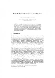
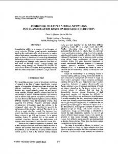
Figure 1: Architecture of the Twin Neural Network However, the TWSVM dual formulation which is conventionally used requires matrix operations such as inversion [8, Eqn (28)-(29)], which is not practical for large datasets due to the size of the data matrix. Further, these operations on large matrices may have issues of numerical stability, which tend to make formulations such as the Twin SVM unsuitable for large datasets. This motivates the need for a neural-network based training algorithm based on the principles of the Twin SVM, that enables effective generalization on large datasets. Another advantage obtained by developing such a framework is that as opposed to the conventional formulation which uses the same kernel function for samples of the two classes, the neural network based approach allows the kernel map to be separately optimized for samples of the two classes, which allows for better generalization.
Twin SVM
Twin Neural Network
· Requires matrix inversion. · Fixed kernel function
· Unsuitable for large datasets.
· Scalable
· Implicit kernel optimization
Figure 2: Comparing TWSVM and Twin NN
2
· Better generalization
Formally, a neural network consists of a set of neurons stacked in an input and output layer, along with single or multiple hidden layers. These neurons are initialized with random weights. As the neural network learns from training samples, the weights are updated using an update rule derived on the basis of error minimization approaches such as gradient descent. Over iterations, these weights converge to their optimal values, allowing efficient prediction on test samples which need to be simply run through the network to obtain class predictions. Intermediate layer neuronal activations are computed using the optimal weights and the final layer arrives at a prediction for the test point. This makes neural networks scalable for large datasets, however it has been found that neural networks often suffer from overfitting and poor generalization ability. In this paper, we propose a neural network formulation motivated by spirit of the TWSVM, whose architecture is summarized in Fig. 1. The objective is to be able to harness the generalization ability of the TWSVM formulation for a neural network, thereby making it scalable for large unbalanced datasets. The added advantage is the inherent optimization of the kernel map separately for the two classes by the layers of the Twin NN. We illustrate this claim by computing the classification accuracy and training time for several large unbalanced datasets. The rest of the paper is organized as follows. Section 2 discusses the formulation for the TWSVM and mentions the dual formulation which is commonly used in practice. Section 3 introduces the Twin Neural Network formulation, followed by Section 4 which shows experimental results to benchmark the performance of the proposed network. Finally, Section 5 presents the conclusions and future work. 2. The Twin Support Vector Machine We begin by motivating the TWSVM from the classical SVM formulation, based on the inability of SVMs to classify unbalanced datasets efficiently. Consider a binary classification dataset of N samples in M dimensions X = {x(1) , x(2) , ..., x(N ) |x(i) ∈ RM , ∀i = 1, 2, ..., N }, with corresponding labels Y = {y (1) , y (2) , ..., y (N ) |y (i) ∈ {−1, +1}, ∀i = 1, 2, ..., N }. We can determine the number of points in each class from the this dataset. Let these be denoted as A = {x(i) |y (i) = +1} for samples of class (+1) and B = {x(i) |y (i) = −1} for samples of class (−1). The soft-margin Support Vector Machine (SVM) classifier has the following formulation. l
min
w,b,ξ
subject to,
X 1 ξi ||w||2 + C 2 i=1
(1)
y (i) (wT (x(i) + b)) ≥ 1 − ξi , ξi ≥ 0, i = 1, . . . , l.
where the separating hyperplane is given by the vector [w, b], C is the upper bound, ξi represents the slack variables for the soft-margin formulation and αi represents the Lagrange multipliers. The SVM finds a maximum margin separating hyperplane for the binary classification dataset. This tends to be biased in cases when the dataset is unbalanced towards the class which has more number of samples. This is undesirable for better generalization on such unbalanced datasets. In order to address this situation, the TWSVM evolved as a viable alternative. The TWSVM determines two non-parallel separating hyperplanes, each of which is as close as possible to points of one class while being at a distance of at least unity from points of the other class. Let these hyperplanes be denoted by the coefficient vectors w(+1) , w(−1) and bias terms 3
b(+1) , b(−1) corresponding to classes (+1) and (−1) respectively. The TWSVM formulation thus involves solving the set of QPPs given by Eqns. (2)-(7).
min
w(+1) ,b(+1) ,q
min
w(−1) ,b(−1) ,q
1 kAw(+1) + e+1 b(+1) k2 + C(+1) eT−1 q, 2 s.t. − (Bw(+1) + e−1 b(+1) ) + q ≥ e−1
q≥0 1 kBw(−1) + e−1 b(−1) k2 + C(−1) eT+1 q, 2 s.t. − (Aw(−1) + e+1 b(−1) ) + q ≥ e+1 q≥0
(2) (3) (4) (5) (6) (7)
Here, data belonging to classes (+1) and (−1) are represented by matrices A[NA ×M ] and B[NB ×M ] respectively, where NA and NB are the number of points in each class such that NA +NB = N . e(+1) and e(−1) are vectors of ones of appropriate dimensions, q represents the error variable associated with the data point and C(+1) , C(−1) (> 0) are hyperparameters. It may be noted here that each of the optimization problems solved for the TWSVM has constraints of only the points belonging to one class, as opposed to the conventional SVM which has points of both classes in the constraints. This makes the TWSVM faster than the conventional SVM. For a test point x, the prediction y is computed by a distance measure based on these two hyperplanes. Essentially, the closer the test point is to one of these hyperplanes, the corresponding class is assigned to it. This is summarized by Eqn. (8).
y=
�
T T +1 : w(+1) x + b(+1) ≤ w(−1) x + b(−1) −1 : otherwise
(8)
In practice, it is more efficient to solve the dual formulation for the TWSVM, which is given by the Eqns. (9)-(10).
max α
s.t. max β
s.t.
1 −1 eT2 α − αT G(H T H) GT α 2 0 ≤ α ≤ c1 1 −1 eT1 β − β T P (QT Q) P T β 2 0 ≤ β ≤ c2
(9)
(10)
Here, H = P = [A, e(+1) ], G = Q = [B, e(−1) ], u = [w(+1) b(+1) ]T , v = [w(−1) b(−1) ]T . As in the case of SVMs, the kernel formulation for the TWSVM is also possible, where the input dataset X is mapped to another feature space (often infinite dimensional) to introduce linear separability in the dataset samples in the mapped feature space. This is typically accomplished using a mapping function denoted by φ(·). The separating hyperplanes are then determined in this mapped space, which is often called as the kernel space. However, it can be seen from the dual formulation of the TWSVM in Eqns. 9-10 that there is a requirement for matrix inversion. This makes it unfeasible for large datasets, where such 4
computations require large memory and are often intractable. Hence, we look for an approach for using the TWSVM within a neural network framework, that would not require such computations thereby making it scalable for large datasets. 3. The Twin Neural Network Formulation We consider a three-layer neural network to motivate the formulation of the Twin Neural Network, as shown in Fig. 1, whose structure is described as follows. The input layer takes the training samples x(i) , i = 1, 2, ..., N and transforms it to a space φ(·) by the neurons of the hidden layer. The final or output layer of this network learns a classifier in the feature space denoted by φ(·), and the classifier hyperplane coefficients (weight vector w and bias b are used to arrive at the prediction for a test sample. For the case of an unbalanced dataset, we propose the formulation of a Twin Neural Network, where two such networks are trained, whose error functions are denoted by E(+1) and E(−1) . These are defined as shown in Eqns. (11)-(12).
E(+1) = +
NA C(+1) X (i) (wT φ(x(+1) ) + b(+1) )2 2 × NA i=1 (+1)
E(−1) = +
NB X 1 (t(i) − y(i) )2 2 × NB i=1
(11)
NA X 1 (t(i) − y(i) )2 2 × NA i=1
NB C(−1) X (i) (wT φ(x(−1) ) + b(−1) )2 2 × NB i=1 (−1)
(12)
To minimize the error, we set the corresponding derivatives to zero to obtain update rules for the weight vector w and bias b. The derivatives w.r.t. w(+1) and w(−1) are shown in Eqns. (13)-(14), which correspond to the weight update rules for our Twin Neural Network. NB ∂E(+1) 1 X (i) 2 = (t(i) − y(i) )(1 − y(i) )φ(x(−1) ) ∂w(+1) NB i=1
+
NA C(+1) X (i) (i) (wT φ(x(+1) ) + b(+1) )φ(x(+1) ) NA i=1 (+1)
(13)
NA ∂E(−1) 1 X (i) 2 = (t(i) − y(i) )(1 − y(i) )φ(x(−1) ) ∂w(−1) NA i=1
+
NB C(−1) X (i) (i) (wT φ(x(+1) ) + b(−1) )φ(x(−1) ) NB i=1 (−1)
5
(14)
Derivatives w.r.t b(+1) and b(−1) are shown in Eqns. (15)-(16), which are used as the update rule for the bias terms in our Twin Neural Network. NB ∂E(+1) 1 X 2 = ) (t(i) − y(i) )(1 − y(i) ∂b(+1) NB i=1
+
NA C(+1) X (i) (wT φ(x(+1) ) + b(+1) ) NA i=1 (+1)
(15)
NA ∂E(−1) 1 X 2 ) (t(i) − y(i) )(1 − y(i) = ∂b(−1) NA i=1
+
NB C(−1) X (i) (wT φ(x(−1) ) + b(−1) ) NB i=1 (−1)
(16)
Based on these, the weights and bias of the hyperplane are updated across the iterations until these hyperplane parameters coverge. The prediction on a test point x is obtained as follows. First, the point is mapped to the space φ(·) by the hidden layer. Then for the output layer, the label y is predicted using Eqn. 17.
y=
(
+1 −1
:
T w(+1) φ(x)+b(+1) ||w(+1) ||
≤
T w(−1) φ(x)+b(−1) ||w(−1) ||
: otherwise
(17)
In terms of machine complexity, it can be shown that the Twin NN formulation minimizes the VC dimension, which results in lower test set errors and hence better generalization. This is in addition to the benefit of scalability obtained as a result of using a neural-network based architecture. Drawing from Burges’s tutorial [4], the VC dimension γ of a classifier with margin d ≥ dmin is bounded by [10] γ ≤ 1 + min(
R2 , n) d2min
(18)
where R denotes the radius of the smallest sphere enclosing all the training samples. T The first Twin NN hyperplane w(+1) φ(x)+b(+1) is similar to Eqn. 19 with the summation taken T over samples of class (+1). Similarly, the second hyperplane w(−1) φ(x) + b(−1) is identical to (19) with the summation taken over samples of class (−1). h=
Max
i=1,2,...M
kuk kxi k ≤
X (uT xi )2
(19)
i
Alternatively, the Twin NN objective function is a measure of the mis-classification error over samples that do not lie in the margin, and is summed over all the training samples of the other class. Hence, the Twin NN objective function tries to minimize a sum of a term that is related to the structural risk, and another that depends on the empirical error. 6
Theorem 1. The Twin NN reduces the total risk by enforcing that an upper bound on the VC dimension is minimized. In effect, note that this is an approximation to the total risk. Vapnik and Chervonenkis [11] deduced, that with probability (1 − η),
Rtotal (λ) ≤ Remp (λ) +
s
η h(ln 2N h + 1) − ln 4 N
N 1 X where, Remp (λ) = |fλ (xi ) − yi |, N i=1
(20) (21)
and fλ is a function having VC-dimension h with the smallest empirical risk on a dataset {xi , i = 1, 2, ..., N } of N data points with corresponding labels {yi , i = 1, 2, ..., N }. 4. Experiments and Discussion 4.1. Results on UCI datasets The Twin NN was tested on 20 benchmark datasets drawn from the UCI machine learning repository [1], which included two class and multi-class datasets. Input features were scaled to lie between -1 and 1. Target set values were kept at +1 and -1 for the respective classes. For multiclass problems, a one versus rest approach [3, pp. 182, 338] was used, with as many output layer neurons as the number of classes. A Twin NN with one hidden layer was employed for obtaining these results. The number of neurons in the hidden layer and the hyperparameters were optimized by using a grid search. The K-Nearest Neighbor (KNN) imputation method was used for handling missing attribute values, as it is robust to bias between classes in the dataset. Accuracies were obtained using a standard 5-fold cross validation methodology. This process was repeated 10 times to remove the effect of randomization. The accuracies were compared with the standard SVM [5], Twin SVM and Regularized Feed-Forward Neural Networks (RFNN) [2]. The results are shown in Table 1, which clearly indicates the superior performance of the Twin NN compared to the SVM, Twin SVM and and RFNN for 15 of the 20 datasets. In addition, we also present a comparative analysis of the performance of the Twin NN on UCI benchmark datasets w.r.t. other approaches in terms of p-values determined using Wilcoxon’s signed ranks test [12]. The values for the Wilcoxon signed ranks test. The Wilcoxon Signed-Ranks Test is a measure of the extent of statistical deviation in the results obtained by using an approach. A p-value less than 0.05 indicates that the results have a significant statistical difference with the results obtained using the reference approach, whereas p-values greater than 0.05 indicate nonsignificant statistical difference. The p-values for the approaches considered are shown in Table 2, which clearly indicates that the Twin NN works better than the reference approaches. To verify that the results on the UCI datasets are independent of the randomization due to the data distribution across folds, we also performed the Friedman’s test [7]. The p-value is 3.77×10⁻¹⁴ (< 0.05), implying that the superior results of the Twin NN are not due to chance, and are clearly a consequence of the approach used rather than the datasets. 4.2. Results on highly unbalanced datasets The key benefit obtained by using the Twin NN is its better generalization for unbalanced datasets. To establish this, we evaluate the Twin NN on several unbalanced datasets [9, 13, 6], which 7
S. No. 1 2 3 4 5 6 7 8 9 10 11 12 13 14 15 16 17 18 19 20
Dataset Pimaindians (768x4) Heartstat (270x13) Haberman (306x3) Hepatitis (155x19) Ionosphere (351x34) Transfusion (748x4) ECG (132x12) Voting (435x16) Fertility (100x9) Australian (690x14) CRX (690x15) Mamm-masses (961x5) German (1000x20) PLRX (182x12) SONAR (208x60) Housevotes (436x16) Balance (576x4) Blogger (100x5) IPLD (583x10) Heart Spectf (267x44)
Lin SVM 76.5 ± 2.99 83.33 ± 4.71 72.22 ± 1.17 80.00 ± 6.04 87.82 ± 2.11 76.20 ± 0.27 84.90 ± 5.81 93.69 ± 0.96 85.03 ± 6.03 85.50 ± 4.04 69.56 ± 0 78.87 ± 2.14 74.1 ± 2.77 71.44 ± 1.06 76.02 ± 6.70 95.88 ± 1.90 94.61 ± 1.68 70.93 ± 12.4 71.35 ± 0.39 78.89 ± 1.02
Ker SVM 77.33 ± 3.15 84.81 ± 3.56 72.32 ± 1.18 83.96 ± 4.05 95.43 ± 2.35 76.60 ± 0.42 87.20 ± 8.48 96.56 ± 1.13 88.03 ± 2.46 86.51 ± 3.96 69.56 ± 0 83.25 ± 3.77 75.20 ± 2.58 72.52 ± 0.44 87.02 ± 6.47 96.56 ± 1.13 99.82 ± 0.38 85.82 ± 8.48 71.35 ± 0.39 79.16 ± 1.23
RFNN 76.11 ± 3.60 81.01 ± 4.82 73.11 ± 2.71 81.11 ± 6.29 86.21 ± 4.28 76.01 ± 1.57 86.25 ± 6.64 94.47 ± 1.90 87.91 ± 6.51 85.24 ± 3.52 68.14 ± 0.94 77.96 ± 2.00 75.8 ± 2.88 71.05 ± 3.54 86.62 ± 6.90 95.56 ± 1.56 97.39 ± 2.39 79.50 ± 9.35 71.05 ± 4.20 79.03 ± 1.17
Twin-NN 78.19 ± 2.73 84.81 ± 2.74 76.11 ± 4.54 86.50 ± 5.98 94.01 ± 1.87 78.07 ± 1.24 91.73 ± 4.75 96.1 ± 1.5 88.03 ± 2.46 87.97 ± 3.89 70.5 ± 1.62 80.75 ± 2.37 76.3 ± 1.35 72.01 ± 1.94 88.53 ± 5.27 97.02 ± 1.00 97.70 ± 1.93 86.01 ± 4.22 73.11 ± 1.64 83.34 ± 3.4
Lin TWSVM 72.99 ± 6.00 83.11 ± 5.86 73.53 ± 0.53 79.11 ± 4.22 85.55 ± 2.93 76.2 ± 0.20 84.32 ± 3.18 93.11 ± 1.41 65.95 ± 3.97 85.71 ± 4.11 65.56 ± 0.34 78.51 ± 1.10 71.99 ± 5.11 72.08 ± 6.7 76.11 ± 3.8 94.61 ± 1.21 94.99 ± 1.7 72.11 ± 1.03 69.97 ± 1.16 78.41 ± 2.17
Ker TWSVM 75.91 ± 6.05 82.49 ± 3.42 73.53 ± 0.53 82.87 ± 1.71 88.92 ± 1.52 76.60 ± 0.42 84.88 ± 2.19 95.32 ± 1.11 88.03 ± 2.46 85.67 ± 1.02 69.57 ± 0 80.11 ± 1.23 72.87 ± 4.71 71.44 ± 1.06 79.35 ± 7.11 96.32 ± 2.71 97.11 ± 2.42 80.87 ± 1.11 71.35 ± 0.48 79.51 ± 1.70
Table 1: Results on UCI datasets for the Twin NN. S.No 1 2 3 4 5
Algorithm Lin SVM Ker SVM RFNN Lin TWSVM Ker TWSVM
p value 8.18E-05 3.80E-02 8.84E-05 1.01E-04 1.31E-04
Table 2: Wilcoxon signed ranks test for the Twin NN are summarized in Table 3. It may be noted here that the class imbalance has been introduced in these datasets by considering the multi-class datasets as separate binary datasets using one-v/srest approach. Thus for a dataset having N classes and M samples per class, we can in principle generate N datasets, each of which has a class ratio of M : (N − 1) · M . Each of these possible datasets has been denoted as “GenN ” suffixed to the dataset name in Table 3, where N represents the corresponding class w.r.t. which imbalance has been induced in the dataset. The procedure to compute the accuracies is illustrated in Fig. 3. For evaluating the performance of the Twin NN on unbalanced datasets, measures other than the classification accuracy are often used in practice. These provide a better understanding of the performance of the learning algorithm taking into consideration the skewness in the dataset. To define these measures, we use four basic quantities, True Positives (T P ), True Negatives (T N ), False Positives (F P ) and the False Negatives (F N ). T P is the number of samples whose class label and predicted label are “true” and T N is the number of samples whose class and predicted labels are “false”. Correspondingly, we use F P for the samples whose class label is “false” and prediced label is “true”, and vice-versa for F N . These are schematically illustrated in the confusion matrix as shown in Fig. 4.
8
Generate unbalanced dataset Divide into 5 subsets for 5-fold cross validation
Train classifier on all-but-one folds. Test on the remaining fold. Repeat 5 times
Compute performance measures. Repeat 10 times. Perform Friedman’s Test
Figure 3: Flowchart for computing accuracy of unbalanced dataset.
S. No. 1 2 3 4 5 6 7 8 9 10 11 12 13 14 15 16 17 18 19 20
Dataset Generated Abalone Gen1 Letter Gen Yeast Gen Abalone Gen2 Coil 2000 Car Eval Gen1 Wine Quality Gen Forest CovType Gen Ozone Level Pen Digits Gen Spectrometer Gen Statlog Gen Libras Gen Optical Digits Gen Ecoli Gen Car Evaluation Gen2 US Crime Gen Protein homology Scene Gen Solar Flare Gen
Source UCI, link UCI UCI UCI UCI KDD UCI UCI UCI KDD UCI UCI UCI UCI UCI UCI UCI UCI UCI KDD CUP 2004 LibSVM Data UCI
Area Life Computer Life Life Business Business Chemistry Nature Environment Computer Physics Nature Physics Computer Life Business Economics Biology Nature Nature
Sample Ratio 1:9 1:26 1:28 1:129 1:15 1:25 1:26 1:210 1:33 1:9 1:10 1:9 1:14 1:9 1:8 1:11 1:12 1:111 1:12 1:19
No of Samples 391 : 3,786 734 :19,266 51 : 1,433 32 : 4,145 586 : 9,236 65 : 1,663 181 : 4,715 2747 : 578,265 73 : 2,463 1,055 : 9,937 45 : 486 626 : 5,809 24 :336 554 : 5,066 35 : 301 134 : 1,594 150 : 1,844 1,296 : 144,455 177 : 2,230 68 : 1,321
Attributes 1N,7C 16 8 8 85 6N, 21 C 11C 44N,10C 72C 16C 93C 36C 90C 64C 7C 6N 122C 74C 294C 10N
Table 3: Description of large unbalanced datasets, attributes are numeric (N) or categorical (C)
9
Predicted Label (+1)
(-1)
TP
FN
FP
TN
(+1) True Label (-1)
Figure 4: Confusion Matrix Based on these, the basic measures are defined as given by Eqns. (22)-(26). Also, P C = T P + F N , N C = F P + T N , P R = T P + F P and N R = F N + T N .
Accuracy (Acc):=
TP + TN TP + TN + FP + FN
(22)
TP TP = TP + FN PC TN TN True Negative Rate (TNR):= = TN + FP NC TP TP Positive Prediction Value (PPV):= = TP + FP PR TN TN Negative Prediction Value (NPV):= = TN + FN NR True Positive Rate (TPR):=
(23) (24) (25) (26)
The performance measure in terms of geometric mean between accuracy of the two classes is called the G-means. This √ is computed as the square-root of the product of the true positive and true negative rates, or as T P R ∗ T N R. The G-means for the unbalanced datasets is shown in Table 4. One can observe that the Twin NN has higher G-means value for all except one dataset when compared to the competing approaches. S. No. 1 2 3 4 5 6 7 8 9 10 11 12 13 14 15 16 17 18 19
Dataset Abalone Gen1 Letter Gen Yeast Gen Abalone Gen2 Coil 2000 Car Eval Gen1 Wine Quality Gen Ozone Level Pen Digits Gen Spectrometer Gen Statlog Gen Libras Gen Optical Digits Gen Ecoli Gen Car Evaluation Gen2 US Crime Gen Protein homology Scene Gen Solar Flare Gen
Twin NN 0.747 ± 0.03 0.95 ± 0.06 0.84 ± 0.04 0.36 ± 0.11 0.66 ± 0.01 1 ± 0.00 0.735 ± 0.07 0.84 ± 0.008 0.9927 ± 0.02 0.956 ± 0.05 0.890 ± 0.011 0.935 ± 0.05 0.991 ± 0.007 0.900 ± 0.06 0.996 ± 0.002 0.85 ± 0.03 0.942 ± 0.006 0.712 ± 0.04 0.705 ± 0.03
Lin SVM 0.045 ± 0.01 0.83 ± 0.05 0.2106 ± 0.09 0±0 0±0 0.934 ± 0.06 0±0 0±0 0.847 ± 0.01 0.902 ± 0.05 0.137 ± 0.04 0.866 ± 0.09 0.888 ± 0.02 0.69 ± 0.11 0.949 ± 0.05 0.635 ± 0.03 0.85 ± 0.01 0.066 ± 0.09 0±0
Ker SVM 0.331 ± 0.14 0.98 ± 0.09 0.411 ± 0.10 0±0 0.031 ± 0.07 0.999 ± 0.001 0.35 ± 0.05 0.283 ± 0.04 0.983 ± 0.06 0.949 ± 0.05 0.745 ± 0.023 0.935 ± 0.05 0.98 ± 0.007 0.78 ± 0.12 0.976 ± 0.04 0.63 ± 0.03 0.89 ± 0.01 0.321 ± 0.06 0±0
RFNN 0.04 ± 0.015 0.88 ± 0.01 0.47 ± 0.12 0±0 0.055 ± 0.05 0.999 ± 0.001 0.245 ± 0.13 0.53 ± 0.06 0.77 ± 0.022 0.938 ± 0.04 0.705 ± 0.023 0.89 ± 0.07 0.964 ± 0.017 0.83 ± 0.06 0.990 ± 0.011 0.69 ± 0.04 0.871 ± 0.006 0.389 ± 0.04 0.29 ± 0.04
Lin TWSVM 0.127 ± 0.02 0.177 ± 0.04 0.20 ± 0.04 0.935 ± 0.04 0.25 ± 0.04 0.187 ± 0.024 0.91 ± 0.07 0.22 ± 0.01 0.821 ± 0.05 0.89 ± 0.01 0.697 ± 0.017 0.934 ± 0.07 0.58 ± 0.01 0.321 ± 0.03 0.35 ± 0.005
Table 4: G-means of large datasets with high unbalance 10
Ker TWSVM 0.358 ± 0.11 0.31 ± 0.06 0.205 ± 0.01 0.955 ± 0.08 0.29 ± 0.01 0.479 ± 0.10 0.950 ± 0.09 0.68 ± 0.01 0.947 ± 0.0 0.952 ± 0.002 0.825 ± 0.01 0.944 ± 0.007 0.65 ± 0.01 0.39 ± 0.01 0.393 ± 0.05
The harmonic mean between the positive prediction value and true positive rate is called the F-measure, which is computed as given by Eqn. (27). F-measure :=
1 TPR
2 +
(27)
1 PPV
The f-measure for the unbalanced datasets is shown in Table 5. From the results, it is evident that the Twin NN has higher f-measure values for all except one dataset, which demonstrates its superior performance. S. No. 1 2 3 4 5 6 7 8 9 10 11 12 13 14 15 16 17 18 19
Dataset Abalone Gen1 Letter Gen Yeast Gen Abalone Gen2 Coil 2000 Car Eval Gen1 Wine Quality Gen Ozone Level Pen Digits Gen Spectrometer Gen Statlog Gen Libras Gen Optical Digits Gen Ecoli Gen Car Evaluation Gen2 US Crime Gen Protein homology Scene Gen Solar Flare Gen
Twin NN 0.358 ± 0.05 0.861 ± 0.02 0.40 ± 0.08 0.02 ± 0.008 0.19 ± 0.01 1 ± 0.00 0.392 ± 0.01 0.42 ± 0.05 0.975 ± 0.01 0.921 ± 0.08 0.67 ± 0.01 0.915 ± 0.04 0.984 ± 0.0007 0.695 ± 0.10 0.958 ± 0.04 0.586 ± 0.04 0.868 ± 0.007 0.337 ± 0.06 0.30 ± 0.03
Lin SVM 0.018 ± 0.005 0.74 ± 0.08 0.092 ± 0.04 0±0 0±0 0.872 ± 0.07 0±0 0±0 0.975 ± 0.01 0.869 ± 0.077 0.04 ± 0.02 0.83 ± 0.10 0.842 ± 0.018 0.57 ± 0.16 0.909 ± 0.07 0.50 ± 0.04 0.8 ± 0.01 0.021 ± 0.009 0±0
Ker SVM 0.065 ± 0.01 0.97 ± 0.06 0.278 ± 0.09 0±0 0.021 ± 0.009 0.99 ± 0.0005 0.206 ± 0.05 0.140 ± 0.03 0.975 ± 0.01 0.915 ± 0.085 0.655 ± 0.02 0.90 ± 0.15 0.983 ± 0.008 0.670 ± 0.15 0.946 ± 0.06 0.497 ± 0.08 0.86 ± 0.01 0.181 ± 0.061 0±0
RFNN 0.0088 ± 0.007 0.852 ± 0.02 0.33 ± 0.13 0±0 0.015 ± 0.0034 0.999 ± 0.0005 0.13 ± 0.08 0.35 ± 0.08 0.743 ± 0.01 0.899 ± 0.08 0.575 ± 0.03 0.88 ± 0.08 0.956 ± 0.018 0.682 ± 0.11 0.95 ± 0.04 0.55 ± 0.04 0.76 ± 0.007 0.207 ± 0.06 0.13 ± 0.02
Lin TWSVM 0.171 ± 0.0007 0.066 ± 0.02 0.015 ± 0.002 0.892 ± 0.004 0.05 ± 0.004 0.091 ± 0.001 0.872 ± 0.089 0.039 ± 0.005 0.81 ± 0.13 0.846 ± 0.019 0.595 ± 0.19 0.89 ± 0.09 0.45 ± 0.07 0.136 ± 0.001 0.15 ± 0.01
Ker TWSVM 0.212 ± 0.01 0.19 ± 0.01 0.0158 ± 0.001 0.937 ± 0.001 0.1 ± 0.001 0.12 ± 0.01 0.918 ± 0.006 0.281 ± 0.01 0.124 ± 0.01 0.886 ± 0.030 0.647 ± 0.15 0.897 ± 0.02 0.56 ± 0.0002 0.182 ± 0.001 0.16 ± 0.005
Table 5: F-measure for large datasets with high unbalance In addition, we also compute the Mathew Correlation Coefficient (MCC) for evaluating the performance of the Twin NN on unbalanced datasets. High MCC values imply that the classifier has high classification accuracy for both classes and also less mis-classification on both classes. The MCC is computed as given by Eqn. 28. The MCC values for the unbalanced datasets is given in Table 6, and the values are higher for the Twin NN for all except two datasets. TP ∗ TN − FP ∗ FN MCC := √ PC ∗ NC ∗ PR ∗ NR
(28)
The p-values for the measures computed on the unbalanced datasets is shown in Table 7. As these values are less that 0.05, they do not indicate significant statistical difference. We also show the average values of the measures computed on the unbalanced datasets in Table 8 for the various approaches. It can clearly be seen that the average values are highest for the Twin NN, indicating its superior performance across the unbalanced datasets. These are also graphically illustrated in Fig. 5. Finally, to illustrate the scalability of the Twin NN on the unbalanced datasets, we present the training time for the Twin NN for these datasets in Table 9. It can be seen that the Twin NN can be trained in tractable time for the unbalanced datasets.
11
S. No. 1 2 3 4 5 6 7 8 9 10 11 12 13 14 15 16 17 18 19
Dataset Generated Abalone Gen1 Letter Gen Yeast Gen Abalone Gen2 Coil 2000 Car Eval Gen1 Wine Quality Gen Ozone Level Pen Digits Gen Spectrometer Gen Statlog Gen Libras Gen Optical Digits Gen Ecoli Gen Car Evaluation Gen2 US Crime Gen Protein homology Scene Gen Solar Flare Gen
Twin NN 0.317 ± 0.05 0.868 ± 0.02 0.41 ± 0.07 0.07 ± 0.02 0.17 ± 0.01 1 ± 0.00 0.41 ± 0.01 0.41 ± 0.05 0.972 ± 0.01 0.92 ± 0.04 0.63 ± 0.02 0.913 ± 0.048 0.981 ± 0.009 0.667 ± 0.11 0.955 ± 0.01 0.552 ± 0.05 0.84 ± 0.01 0.282 ± 0.06 0.262 ± 0.09
Lin SVM 0.019 ± 0.04 0.761 ± 0.03 0.12 ± 0.16 0±0 (-)0.0011 ± 0.002 0.871 ± 0.069 (-)0.001 ± 0.002 (-)0.0015 ± 0.003 0.775 ± 0.02 0.863 ± 0.08 0.113 ± 0.05 0.83 ± 0.10 0.828 ± 0.018 0.540 ± 0.14 0.902 ± 0.07 0.50 ± 0.04 0.83 0.01 0.061 ± 0.09 0±0
Ker SVM 0.05 ± 0.13 0.97 ± 0.006 0.372 ± 0.068 0±0 0.017 ± 0.05 0.995 ± 0.001 0.27 ± 0.06 0.204 ± 0.066 0.968 ± 0.01 0.91 ± 0.08 0.63 ± 0.02 0.91 ± 0.09 0.981 ± 0.009 0.64 ± 0.16 0.945 ± 0.07 0.51 ± 0.06 0.86 ± 0.01 0.25 ± 0.06 0±0
RFNN 0.043 ± 0.059 0.851 ± 0.02 0.38 ± 0.10 0±0 0.03 ± 0.04 0.999 ± 0.001 0.19 ± 0.11 0.343 ± 0.08 0.752 ± 0.018 0.89 ± 0.08 0.542 ± 0.03 0.885 ± 0.08 0.952 ± 0.019 0.690 ± 0.13 0.945 ± 0.04 0.53 ± 0.03 0.79 ± 0.01 0.190 ± 0.08 0.14 ± 0.11
Lin TWSVM 0.08 ± 0.06 0.08 ± 0.07 0±0 0.851 ± 0.01 0 ± 0.05 0.01 ± 0.13 0.852 ± 0.09 0.09 ± 0.05 0.80 ± 0.11 0.826 ± 0.009 0.587 ± 0.09 0.884 ± 0.09 0.497 ± 0.1 0.131 ± 0.09 0±0
Ker TWSVM 0.125 ± 0.03 0.21 ± 0.08 1±0 0.94 ± 0.04 0.05 ± 0.02 0.052 ± 0.05 0.911 ± 0.05 0.481 ± 0.01 0.0 ± 0.00 0.839 ± 0.03 0.61 ± 0.17 0.908 ± 0.03 0.511 ± 0.08 0.15 ± 0.001 0±0
Table 6: MCC for large datasets with high unbalance S.No 1 2 3
Algorithm Linear SVM Kernel SVM RFNN
G-Means 1.32E-04 5.36E-04 1.32E-04
F-measure 1.96E-04 1.17E-03 1.36E-04
MCC 1.31E-04 5.61E-03 2.92E-04
Table 7: p-values for Wilcoxon signed ranks test for different measures on unbalanced Datasets Average G-Means F-Measure MCC
Linear SVM 0.465768 0.425158 0.421547
Kernel SVM 0.609421 0.539605 0.551684
RFNN 0.607684 0.5272 0.533789
Twin NN 0.842195 0.651632 0.612053
Table 8: Average Values of G-Means, F-Measure, MCC and AUC for Unbalanced Datasets S. No. 1 2 3 4 5 6 7 8 9 10 11 12 13 14 15 16 17 18 19
Dataset Generated Abalone Gen1 Letter Gen Yeast Gen Abalone Gen2 Coil 2000 Car Eval Gen1 Wine Quality Gen Ozone Level Pen Digits Gen Spectrometer Gen Statlog Gen Libras Gen Optical Digits Gen Ecoli Gen Car Evaluation Gen2 US Crime Gen Protein homology Scene Gen Solar Flare Gen
Twin NN 0.292 ± 0.09 5.01 ± 0.98 0.32 ± 0.1 2.1 ± 0.1 20.1 ± 2.2 0.8 ± 0.06 4.2 ± 0.8 2.9 ± 0.06 4.38± 0.29 0.31± 0.03 5.21± 0.9 0.50± 0.007 9.18± 0.30 0.15± 0.01 0.61± 0.01 3.8± 0.23 132.2± 2.87 6.2± 1.01 0.20± 0.03
Lin SVM 0.55 ± 0.008 15.01 ± 0.45 0.03 ± 0.0001 0.06 ± 0.002 22.67 ± 0.18 0.07 ± 0.002 1.8 ± 0.007 0.6 ± 0.02 6.79± 0.29 0.09± 0.008 5.35± 0.1 0.69± 0.011 10.30± 005 0.01± 0.0008 0.13± 0.005 0.89± 0.03 235.12± 8.19 6.6± 0.11 0.10± 0.006
Ker SVM 1.08 ± 0.02 19.47 ± 0.49 0.09 ± 0.001 0.14 ± 0.001 27.06 ± 0.2 0.5 ± 0.004 2.1 ± 0.05 1.51 ± 0.008 9.36± 0.48 0.10± 0.003 5.61± 0.5 0.75± 0.02 20.53± 0.17 0.05± 0.001 0.60± 0.009 2.05± 0.02 744.78± 32.71 11.9± 0.09 0.23± 0.008
RFNN 1.05 ± 0.38 6.88 ± 1.85 1.08± 0.15 1.7 ± 0.09 21.22 ± 4.21 0.6 ± 0.009 2.1 ± 0.05 1.98 ± 0.09 4.68± 0.12 0.58± 0.18 5.91± 0.5 0.63± 0.11 9.87± 0.33 0.40± 0.1 0.59± 0.05 1.84± 0.27 188.2±5.22 10.03± 0.24 0.63± 0.07
Table 9: Training time for unbalanced datasets
12
Lin TWSVM 104 ± 7.58 14.28 ± 0.53 132 ± 13 8.36 ± 0.067 28.11± 0.92 21.88 ± 2.7 0.60± 0.07 55.97± 1.87 0.24± 0.008 65.72± 1.79 0.21± 0.001 11.85± 0.02 27.83± 7.82 32.60± 0.79 3.77± 0.6
Ker TWSVM 231 ± 9.11 35.27 ± 1.89 255 ± 8.72 24.11 ± 1.17 117.64± 5.43 114.5 ± 4.7 4.81± 0.21 127.97± 2.88 1.13± 0.01 132.72± 3.21 1.08± 0.08 50.34± 1.75 56.87± 0.91 137.46± 7.48 8.7± 1.1
Figure 5: Average Values of G-Means, F-Measure, MCC and AUC for Unbalanced Datasets. 4.3. Experiments on scalability We analyze the scalability of the Twin NN on the Forest Covertype dataset described in Table 10. The dataset with imbalance generated has an imbalance ratio of 1 : 211, with 44 numeric and 10 categorical attributes. Dataset Generated Source Area Imbalance Ratio Number of Samples per class Attributes Original Dataset Original Classes Class No. used to generate imbalance
Forest CovType Gen UCI KDD Nature 1:211 2747 : 578,265 44N,10C Forest CovType 7 4
Table 10: Dataset for scaling experiment The performance parameters for this case have been shown in Table 11 for various number of training samples, and the corresponding training time has been shown in Table 12. These are also graphically illustrated in Fig. 6. It can be seen that in comparison to the other methods, the Twin NN scales well and also trains in tractable time with increase in number of training samples. This establishes the scalability of the Twin NN for imbalanced datasets.
13
Train Data Size 116202 232404 348606 464808 116202 232404 348606 464808 116202 232404 348606 464808
TNN SVM Linear G-means values 0.9627 0.017 0.9689 0.112 0.9731 0.1754 0.9802 0.3857 F-measure 0.7581 0.01 0.7881 0.051 0.8172 0.0653 0.8172 0.2485 MCC values 0.7611 0.041 0.7911 0.112 0.8162 0.1649 0.8198 0.3382
SVM Kernel
NNREG
0.7712 0.8132 0.8361 0.8391
0.54 0.57 0.5808 0.5885
0.72 0.771 0.8069 0.8071
0.41 0.43 0.467 0.4736
0.74 0.78 0.8154 0.8196
0.4523 0.4512 0.5464 0.5487
Table 11: Performance parameters for scaling experiment Train Data Size 116202 232404 348606 464808
TNN 89.48 149.38 209.41 385.93
SVM Linear 338.8 990.4 3129.21 6254.1
SVM Kernel 1290.11 5811.32 28716.11 41861.21
NNREG 91.11 181.27 227.41 394.71
Table 12: Training Time for scaling experiment
5. Conclusion and Future Work This paper presented the Twin Neural Network, which provides a neural network training algorithm which minimizes machine complexity in terms of VC dimension and overcomes the issue of scalability of the Twin SVM. The Twin NN has been shown to have superior performance on several datasets, particularly for the case of unbalanced datasets. Acknowledgements The corresponding author would like to acknowledge the support of the Microsoft Chair Professor Project Grant (MI01158, IIT Delhi). References [1] Arthur Asuncion and David Newman. Uci machine learning repository, 2007. [2] George Bebis and Michael Georgiopoulos. Feed-forward neural networks. Potentials, IEEE, 13(4):27–31, 1994. [3] Christopher M Bishop. Pattern recognition and machine learning. springer, 2006. [4] Christopher JC Burges. A tutorial on support vector machines for pattern recognition. Data mining and knowledge discovery, 2(2):121–167, 1998. 14
Figure 6: Average Test Values of G-Means, F-Measure, MCC and AUC and Training Time for Scaleup Experiment.
15
[5] Chih-Chung Chang and Chih-Jen Lin. Libsvm: A library for support vector machines. ACM Transactions on Intelligent Systems and Technology (TIST), 2(3):27, 2011. [6] Zejin Ding. Diversified ensemble classifiers for highly imbalanced data learning and their application in bioinformatics. 2011. [7] Milton Friedman. The use of ranks to avoid the assumption of normality implicit in the analysis of variance. Journal of the American Statistical Association, 32(200):675–701, 1937. [8] Jayadeva, Khemchandani R., and Chandra S. Twin Support Vector Machines for pattern classification. Pattern Analysis and Machine Intelligence, IEEE Transactions on, 29(5):905– 910, 2007. [9] Miroslav Kubat, Robert C Holte, and Stan Matwin. Machine learning for the detection of oil spills in satellite radar images. Machine learning, 30(2-3):195–215, 1998. [10] Vladimir N Vapnik. Statistical learning theory. 1998. [11] Vladimir N Vapnik and A Ja Chervonenkis. Theory of pattern recognition. 1974. [12] Frank Wilcoxon. Individual comparisons by ranking methods. Biometrics bulletin, pages 80–83, 1945. [13] Kevin S Woods, Chiristopher C Doss, Kevin W Bowyer, Jeffrey L Solka, Carey E Priebe, and W Philip Kegelmeyer JR. Comparative evaluation of pattern recognition techniques for detection of microcalcifications in mammography. International Journal of Pattern Recognition and Artificial Intelligence, 7(06):1417–1436, 1993.
16