1236
IEEE TRANSACTIONS ON CIRCUITS AND SYSTEMS—I: REGULAR PAPERS, VOL. 52, NO. 6, JUNE 2005
Neural Network Approach to Blind Signal Separation of Mono-Nonlinearly Mixed Sources W. L. Woo, Member, IEEE, and S. S. Dlay, Member, IEEE
Abstract—A new result is developed for separating nonlinearly mixed signals in which the nonlinearity is characterized by a class of strictly monotonic continuously differentiable functions. The structure of the blind inverse system is explicitly derived within the framework of maximum likelihood estimation and the system culminates to a special architecture of the 3-layer perceptron neural network where the parameters in the first layer are inversely related to the output layer. The proposed approach exploits both the structural and signal constraints to search for the solution and assumes that the cumulants of the source signals are known a priori. A novel statistical algorithm based on the hybridization of the generalized gradient algorithm and metropolis algorithm has been derived for training the proposed perceptron which results in improved performance in terms of accuracy and convergence speed. Simulations and real-life experiment have also been conducted to verify the efficacy of the proposed scheme in separating the nonlinearly mixed signals Index Terms—Independent component analysis (ICA), neural networks, nonlinear distortion, nonlinear systems, signal reconstruction.
I. INTRODUCTION
I
N RECENT TIMES, blind source separation (BSS) using independent component analysis (ICA) has received attention because of its potential application in signal processing such as in speech recognition systems, telecommunications and medical signals processing. The goal of ICA is to recover independent sources given only sensor observations that are unknown linear mixtures of the unobserved independent source signals. Many if not complete theories regarding various aspects of the linear BSS have been established and confirmed experimentally [1], [2]. However, in general, and for many practical problems, mixed signals are more likely to be nonlinear or subject to some kind of nonlinear distortions due to sensory or environmental limitations. For example, in medical imaging systems, the magnetic resonance and computed tomography are strongly affected by artifacts and nonlinearities which are generated from many independent sources [3]. In some signal and array processing applications, the components and sensor elements often exhibit nonlinear behavior at certain signaling conditions [4], [5]. In each case, there is an urgent need to be able to identify these nonlinearities and more importantly, ameliorate their effects in order to obtain a clear and accurate representation of the actual signals.
Manuscript received August 28, 2003; revised June 29, 2004 and October 7, 2004. This paper was recommended by Associate Editor Y. Inouye. The authors are with the School of Electrical, Electronic and Computer Engineering, University of Newcastle upon Tyne, Newcastle upon Tyne, NE1 7RU, U.K. (e-mail:
[email protected]). Digital Object Identifier 10.1109/TCSI.2005.849122
II. NONLINEAR MIXING MODEL There have been increasing number of real-life applications involving the use of nonlinear models and as a result, the need to acquire nonlinear control algorithm has become a crucial part of the signal processing design. In this paper, a nonlinear model based on the theory of functional analysis [23] for modeling nonlinear mixtures is derived. The following lemma establishes the foundation upon which the model can be derived. Lemma 1 [23]: If an equation can be expressed in the form of where one of the funcof tions (or ) is a continuous group operation for the , an interval, then equation has a strictly monotonic continuous function if and only if the other function (or ) is also a continuous group operation. On applying Lemma 1, if two source signals (e.g., and ) and and are related to the function as the group operation is defined as where is simply an arbitrary scalar whose range is bounded , then the group operation within [ , 1] i.e., will assume the form of
and the auto-associative operation
Moreover, we may generalize the group operation three elements as follows:
to include
(1) and . Following identical procedure as in (1), this can be extended to include number of elements as . Now, if a nonlinear system with inputs and outputs can be defined as with where (set where
1057-7122/$20.00 © 2005 IEEE
WOO AND DLAY: NEURAL NETWORK APPROACH TO BLIND SIGNAL SEPARATION
of positive integers), input source signal, it then follows that
and
is the th
(2) where
Therefore, the nonlinear system can be described by the following model:
.. .
.. .
.. .
(3)
where with dimension with . Eriksson and Koivunen [24] also arrived at the same model in (3). Our emphasis is on the relation of the duality nature between group operation and function equivalence in Lemma 1 with the general nonlinear source mixture model in (2). In direct contrast with our proposed method, [24] conto be known a priori at the siders the nonlinear functions demixing stage which eventually render their developed algoare rithm nonblind. In the proposed method, the functions unknown except that they are constrained to be strictly monotonic and continuously differentiable. In addition, if the noncan assume the form of linear mapping functions , then (3) reduces to a “mono-nonlinearity” . The objective of the model exemplified by proposed work is to estimate the unknown nonlinear function and subsequently used in conjunction with other method to restore the input source signals that have been nonlinearly mixed by the mono-nonlinearity system. The number of sources can be estimated by some kind of pre-processing subspace techniques as investigated by Cardoso [25] or by using a more principled approach based on Bayesian framework as investigated by Lappalainen and Miskin [26]. We note that Lemma 1 together with (1)–(3) aim to point out the relation of the duality nature between group operation and function equivalence with the general nonlinear source mixture. Invoking the universal approximation theorem [27], there ex-
1237
such that the group operator as govists erned by the mapping function , which assumes the form of a strictly monotonic continuous function can be approximated by . a simple perceptron with the structure is hidden layer nonlinearity chosen a priori while Here, , and are the unknown variables to be determined during the learning process. The following theorem shows how the perceptron can be used for approximating the model in (3). in (3) be Theorem 1: Let the mapping function constrained to a class of strictly monotonic continuous (if is a scalar function) or continuously differentiable (if is a vector function) with assuming the form of a nonconstant, bounded, monotonically increasing function. Hence, can be represented the inverse of the mapping function by where the superscript “ ” represents the pseudoinverse. Thus, the nonlinearly mixed signals can be approximated according to where . Note that the vector mapping function can if be transformed to a scalar mapping and are diagonal matrices. In addition, if the function is differentiable with respect to its argument and that at an arbitrary point , then there exist where , such open sets onto . In addition, when that is a diffeomorphism of is smooth, then the inverse mapping is also a smooth diffeomorphism such that and comprise a unique one-to-one local mapping on and . Assuming that with square and invertible and , hence we have where is the element by ele, i.e., . ment first order derivative1 of Since the Jacobian determinant of the derivative matrix must be strictly nonzero for at least a locally invertible unique solution to exist, then must hold which implies that for all . Now, as the mapping function is given by a continuously differto be conentiable function, this stringently requires that tinuous at all points and be defined at every point in the open set of the input space. The ideal candidate is the sigmoid function which belongs to the class of continuously differentiable function and possesses the characteristics of nonconstant, bounded and monotonically increasing. Besides, sigmoid function is a bijective mapping so that the existence of a differentiable continuous inverse function is always warranted which is required for . Thus, the nonlinear mixing system the approximation of can be approximated using a general perceptron model with inas vertible
(4) in the second line of where we have substituted (4). Of special note is that in the universal approximation formuand can be nonsquare matrices. Thus, this results lation,
1238
IEEE TRANSACTIONS ON CIRCUITS AND SYSTEMS—I: REGULAR PAPERS, VOL. 52, NO. 6, JUNE 2005
in the inverse function obtained by inverting the perto have lesser accuracy. ceptron parameters as In spite of this, it is shown in Appendix A that will still hold but only at points given by the column span of . Thus, is locally invertible. On the other hand, are constrained to be square invertible matrices, if although at the expense of trading off the approximation acis better approximated by curacy, the inverse function than if and were to be nonsquare matrices. This implies that there is a tradeoff in approximaand tion accuracy between the simultaneous estimation of . In both cases, in (4) is obtained only in an approximate manner. Equation (4) suggests that any nonlinear system satisfying Lemma 1 and is governed by strictly monotonic continuously differentiable functions can be approximated by a constrained 3-layer perceptron where the first layer is inversely related to the output layer. Theorem 2: The maximum likelihood estimate of the source signals under the assumption of gaussian additive noise for the mixing system in (4) with satisfying Theorem 1 is given by (5) where
is the constraint constructed from the a priori information about the source signals and is the scalar constant chosen to provide the required amount of weighting on the con” denotes the cumulant operator straints. The symbol “ of a random variable . We assume that the cumulants of the sources are known. These cumulants will be used to resolve the indeterminacy of the scale generated by the likelihood solution to the mono-nonlinearity mixture. For the computation of cumulants, readers are referred to [28]. Since the output of the nonlinear system depends only on the current source signal and not any previous temporal information, the conditional log likelihood reduces to which allows us to express c-ML cost function as
(9)
At the limit
, (9) can be written as
. (Proof: See Appendix B). III. NONLINEAR DEMIXING MODEL
A. Estimation of the Nonlinear Inverse System Parameters For separating nonlinearly mixed signals, we propose a 3-layer perceptron that closely mimics the desired solution established in (5). The input–output relationship of the proposed 3-layer perceptron is given as
(6) is the adjoint of . In vector form, this can where with be written as and . The paramewill be trained using a parametric approach ters based on the constrained maximum likelihood (c-ML) given by
(10) Source separation in a nonlinear mixing system is fundamentally an ill-posed problem as demonstrated by the fact that the existence of unique inverse solution is usually violated. A natural way of regularizing the solution consists in looking for . To separating mappings belonging to a specific subspace , characterize the indeterminacies for this specific model Jutten and Karhunen [22] suggests to examine the independence preservation equation which states that for all within where is a -algebra on , there exists (11) Denoting as the set of transforms that preserve independence and as the set
(12) (7) (8)
In the above, is set of parameters of the 3-layer perceptron while and denote the collection of observations and final outputs of the perceptron, respectively with and . The term
of all source signal distributions for which there exists a nontrivial mapping belonging to the model and preserving the independence of the components of the input vector . Ideally, should be empty and should contain the permutation matrix as the unique element. Unfortunately, in a general nonlinear mixing system this is not fulfilled and the source signals can be restored up to an belonging to the set invertible transformation [22], [29]. However, in the proposed mono-nonlinearity mixing system, it is possible to correctly extract the true source signals provided that the following conditions are satisfied. Let the nonlinear inverse system be given by a feedforward multilayer
WOO AND DLAY: NEURAL NETWORK APPROACH TO BLIND SIGNAL SEPARATION
1239
c-ML can be iteratively solved by using the generalized gradient ascent method
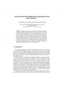
Fig. 1. Combined mixing-inverse system.
perceptron (FMLP) with two hidden layers of nonlinearity which may be abstractly represented as where is an arbitrary nonsingular matrix, and are two continuously differentiable functions such that . The combined nonlinear mixing-inverse system is shown in Fig. 1. Suppose that has independent elements where, at most, only one Gaussian element and that each element accepts a density function that vanishes at one is a nonsingular square matrix with point. Also suppose that at least two nonzero entries per row or per column and is a differentiable invertible function. Under these conditions, it is also independent can be shown that and provided that where is a nonzero scalar, is a constant vector, is a permutation matrix and is a nonzero diagonal matrix according to the Fig. 1, it follows that [15]. Since . Following from and , and hence, this the result shows that to be related to as . enables and , the output of Having established the functions inverse system may now be related to the source signals as
(14) is the pdf of the th output of the network which where is unknown and need to be estimated. The gradient of the c-ML have with respect to the network parameters been derived as follows (see Appendix C):
(15) (16) (17) where
and
. Amari [30] proposes to replace the standard steepest gradient with the natural gradient algorithm which is based on differential geometry whereby the Riemannian metric tensor is automatically incorporated into can be the algorithm. The natural gradient algorithm for implemented as follows:
(13) (18) are the indeterminacy where , and associated with the solution to the mono-nonlinearity mixing model obtained using the independence criterion. Hence, we can accurately recover the original source signals up to a permutation if and only if and . As mentioned above, we by using the signal constraint in (9). Since can force has at least two nonzero entries per row or per column, the term can never equate to a zero vector and therefore, can be satisfied if and only if for any nonzero . Of special interest is the relation of (4) with the post-nonlinear (PNL) mixture [15]. One key difference between these two models is that we can accurately recover in the mono-nonand whereas linearity mixing model if and only if no such constraints are necessary in the PNL mixture.
(19) The mathematical theory of the natural gradient algorithm is currently unfounded in the literature of nonlinear signal separation but previous experimental studies [16], [19], [20] have already been undertaken and meticulously conducted within this work which enabled us to verify its efficacy in improving the convergence rate of the parameters adaptation. Besides, when is a square matrix, the natural gradient algorithm in (19) alto be updated without having to compute the inverse lows matrix as in (16) which subsequently reduces the overall computational complexity. C. Hybrid Gradient-metropolis Learning Algorithm
B. Derivations of the Learning Algorithm In the derivation of the learning algorithm, we have adopted a general approach where and can be square or nonsquare matrices. In the results, we focus only on the square matrices. Using the instantaneous estimate of the statistics, the
The generalized stochastic gradient algorithm exemplified in (17)–(19) searches for the solution in a multidimensional space along the steepest ascent direction. Such a search can be extremely slow and ineffective if the c-ML has many plateaus distributed throughout the landscape or when the algorithm
1240
IEEE TRANSACTIONS ON CIRCUITS AND SYSTEMS—I: REGULAR PAPERS, VOL. 52, NO. 6, JUNE 2005
is trapped in local maxima. In such cases, statistical search methods may offer better strategy in ameliorating both problems. One of the most widely used statistical search method is the simulated annealing [31] which uses the metropolis algorithm to decide whether to accept or reject a configuration that results in an increased error during its attempts in searching for the minimum error configurations in a combinatorial problem. Simulated annealing procedure has also been previously applied to BSS problem [32], [33]. There are however a few issues to be aware of, particularly that the simulated annealing is not so proficient in fine tuning the optimum solution even after locating an appropriate region in the solution space whereas gradient algorithms exhibit good performance only in local optimization. In addition, the convergence of the annealing process is mainly controlled by the operating temperature which must be gradually adjusted impacting in extremely slow rate of convergence in the overall learning scheme. Moreover, since the search space is enormously vast, the randomization that occurs during the perturbation process of the metropolis algorithm may result in unproductive attempts in searching along incorrect directions. Therefore, a hybrid learning algorithm that combines both metropolis and gradient ascent algorithms is devised in order to incorporate the merits of both methods. This new approach employs the statistical operator as a searching tool for the gradient method to acquire a quicker trajectory in learning the optimal solution during the adaptation phase. This is advantageous when the gradient ascent algorithm is trapped at a local maximum or that the convergence rate is relatively small due to the convergence to plateaus resulting in the average rate of change of the cost function dropping within a particular range, which will then activate the statistical search by randomly perturbing the values of the current network parameters to generate some new values. The algorithm then chooses the values of the parameters that optimize the cost function according to the probabilistic rules crafted by the metropolis algorithm. Commencing from the new network configuration, the parameters will be adapted by the gradient ascent algorithm until it converges to the global solution. These procedures are repeated whenever the gradient method converges to another local maximum or the convergence rate is found to be too small at a regular interval. The perceptron learning algorithms based on the hybridization of metropolis algorithm and generalized gradient algorithm are outlined as follows. , Step 1) Initialize . from (6), Step 2) Compute from (14) and
perature and is a random number selected from a [0,1] uniform distribution. . Else Step 5) Return to Step 2 until . As the main aim of the metropolis algorithm is to stimulate global convergence of the hybrid algorithm, the selection of the correct operating temperature is vital. The operating temperature should follow a scheme whereby it can be easily inferred whenever the hybrid algorithm converges to local maxima or plateaus. The process of selecting can be achieved as follows: Since the term measures the average rate of change in conwill fluctuate in vergence of the proposed algorithm, then the vicinity close to zero whenever the algorithm converges to local maxima or plateaus. Therefore, the operating temperature should be selected inversely proportional to the average rate of where and are change as given by some positive constants. This ensures that whenever Step 4 is to relate the visited the algorithm uses the information average rate of change in convergence with the magnitude of the operating temperature so as to allow high probability of relocation once convergence to local maxima or plateaus is apparent. As with other blind algorithms, convergence to global solution is not always guaranteed using gradient or statistical search methods. However, statistical search methods are more likely to find the global solution than the gradient methods. We show by simulations and real-time experiment that the proposed hybrid method is effective in separating nonlinearly mixed signals. IV. RESULTS As a performance measure, conventional signal processing techniques use the mean square error (MSE) criterion to characterize the efficacy of the performance. However, MSE criterion is sensitive to the variability of both scale and phase of the recovered signal. In the context of signal separation, the recovered signal can be subject to scale and phase reversal ambiguities and therefore, the MSE criterion is not suitable for performance comparison among different algorithms. As an alternative, we propose the following performance index: (20) where (21) .
, use natural gradient algorithm via Step 3) If (17)–(19) to update . and , activate the statisStep 4) If to generate tical search method by perturbing and proceed as follows: a new state If , then . for , then Elseif where is the operating tem-
where is the th final output of the perceptron at time and is the normalized cross-correlation. In above, “ ” and “ ” denote the complex conjugate and absolute operation, respectively. The proposed performance index is essentially a variant of the MSE criterion that implicitly takes into account the scale and phase reversal ambiguities (see Appendix D). It is desirable to have the performance index as small as possible as this represents the achieved accuracy of the nonlinear inverse system
WOO AND DLAY: NEURAL NETWORK APPROACH TO BLIND SIGNAL SEPARATION
1241
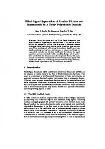
Fig. 2. Signals for experiment 1. (a) Original sources. (b) Linear ICA. (c) RBF. (d) Valpola’s method. (e) Proposed method. (f) Performance index.
in restoring the original signals. In all experiments, the number of hidden neurons used in the proposed algorithm is identical to the number of sources. A. Experiment 1 In this experiment, the following nonlinear mixture for the case of three source signals and three sensors is considered since such study can assists us in gaining insights into the efficacy of the proposed scheme. The source signals are nonlinearly coupled according to a third order system given by
(22)
, and are the source where signals, observed signals and noise, respectively. By the application of Lemma 1, there exist and which are both strictly monotonic continuously differentiable functions and substituting these functions into (22), the latter can be represented as the mono-nonlinearity mixing system as
(23)
, is the matrix sandwiched between where the two layers of nonlinearity and . where The sources are given by , and is a uniformly distributed random signal and each dB white gaussian noise. sensor is perturbed with The perceptron in (7) with three input nodes, three hidden as nodes, three output nodes and the hidden function is used as the nonlinear inverse system. The observed signals are first partitioned into blocks of 32 samples and then fed to the demixer where the parameters are updated in a block-by-block manner. The parameters of the perceptron are randomly initialized with the step sizes chosen to be 0.01, , , , . These initial values have been repeatedly performed on various experiments and the results obtained have confirmed the validity of the usage of such values. The original source signals are shown in Fig. 2(a). Concurrently, we compare the attained best performance with three existing schemes: Linear ICA [34], radial basis function (RBF) with three input nodes, 15 hidden nodes and three output nodes [9] and Valpola’s method using 2-layer perceptron with three input nodes, 12 hidden nodes and three output nodes [14]. In linear ICA, the demixer is initialized with identity matrix and the step sizes of 0.01 is used to update the weights and the statistical parameters of the estimated signals. In RBF, the linear weights initialized with identity matrix, the step sizes for updating both the width of the Gaussian neuron and the weights are set to 0.01 while centre of the Gaussian neuron is trained using the enhanced -means clustering algorithm. In Valpola’s method, the inferred mixing model is represented as where is the sensor noise and , and are the parameters of the model. The aim of Valpola’s
1242
Fig. 3.
IEEE TRANSACTIONS ON CIRCUITS AND SYSTEMS—I: REGULAR PAPERS, VOL. 52, NO. 6, JUNE 2005
Signals for experiment 2. (a) Original sources. (b) Linear ICA. (c) RBF. (d) Valpola’s method. (e) Proposed method. (f) Performance index.
method is to determine by inferring , , , from the observed signals. Fig. 2(b)–(e) shows the recovered signals of the four schemes while Fig. 2(f) the achieved performance index under various signal-to-noise ratios (SNR). From the plots, it is clearly identified that the proposed method has outperformed the three schemes across the range of SNRs and that the performance attained by the linear ICA falls far from being optimum which points out the insufficiency of using linear model. The poor performance of the linear ICA approach can be attributed to the fact that it does not satisfy the linear separability condition [35] when the mixing system is embedded in nonlinearity. As for the RBF, we first note that the mixing is governed by the mono-nonlinearity system which consists of two layers of nonlinearity but the RBF demixer has only 1 layer of nonlinearity and hence, there is a strong structural mismatch between the mixing and demixing models. Hence, the RBF will be unable to compensate for the nonlinearity in the mixing model. In addition, the mixing nonlinear function is global but RBF demixer uses a local function given by the Gaussian function and as a result, the RBF demixer tends to produce smooth estimates of the source signals. As for Valpola’s method, there is also the problem of structural mismatch but it is seen that the separated signals closely resemble the original source signals. Careful inspection on the signal waveforms reveals that the separated signals are not truly the source signals but are nonlinearly distorted version of the latter. The reason is that Valpola’s method uses a 2-layer perceptron and this enables the demixer to equalize the effects of the outer layer nonlinearity and the mixing matrix . However, since Valpola’s method uses the Kullback–Leibler divergence as the cost function, it cannot distinguish whether the extracted outputs are in the form
. Therefore, the extracted outputs are identical to of or the source signals subject to a one-to-one nonlinear distortion. B. Experiment 2 Here, a set of five source signals is passed through the following nonlinear mixing model: (24) , and are where represents the sensor noise and 5 5 randomly sampled full rank matrices. Two types of nonlinearities will be considered. The first type of nonlinearity will be given by a third-order odd polynomial function in the form and the second type is given by its inof verse form which can be expressed in the following closed form function: (25)
where
. The
parameter controls the amount of nonlinearity of the function. The main impetus of this experiment is to examine the robustness of the proposed solution to the deviations from the mixing model in terms of both functional and structural mismatches. , The source signals are given by , , and is a uniformly distributed random signal. These signals are plotted in Fig. 3(a). This experiment
WOO AND DLAY: NEURAL NETWORK APPROACH TO BLIND SIGNAL SEPARATION
Fig. 4.
1243
Signals for experiment 3. (a) Original sources. (b) Observed mixed signals. (c) Linear ICA. (d) RBF. (e) Valpola’s method. (f) Proposed method.
aims to investigate the robustness of the proposed method under functional mismatch of different nonlinearity in each while channel and this is carried out by selecting and to be the corresponding first and second layer of nonlinearity. In each layer, the nonlinearity parameter is set according to , , , and such that describes a variable degree of nonlinearity. As each a consequence, and this results in the departure from the mono-nonlinearity mixing structure in (4). Linear ICA, RBF, Valpola’s method, and the proposed method are used as the demixing systems. The RBF demixer uses five input nodes, 25 hidden neurons and five outputs while Valpola’s 2-layer perceptron uses five input nodes, 20 hidden neurons, and five outputs. Similar parameter settings used in experiment one are adopted for each system. The performance of signal separation is illustrated in Fig. 3(b)–(e), while Fig. 3(f) shows the performance index of each tested scheme. Despite the structural mismatch between the mixing model and the proposed scheme, a high degree of performance gain over other methods is perceivable from the proposed scheme. C. Experiment 3 In this experiment, real-life speech mixture is used which is recorded by three carbon-button microphones. We allow the recording amplifier to operate in the saturation region [36]. Moreover, the secondary cause of nonlinearities could arise from the nonuniform flux of the permanent magnet and the
nonlinear response of the suspensions in the loudspeaker. In addition, the carbon-button microphones may exhibit some form of memoryless nonlinearities and, therefore, contribute further to the distortion of the signals [37]. The recorded signals are then sampled at 24 kbit/s and are displayed in Fig. 4(a) along with the received signals at the output to the microphones in Fig. 4(b). Similar parameter settings as in the first experiment are used except that the step sizes are now changed to 0.005 . and that the perceptron learning process is based on Three learning algorithms are used to update the parameters of the proposed perceptron: 1) conventional gradient ascent algorithm; 2) natural gradient ascent algorithm; and 3) Hybrid natural gradient-metropolis ascent algorithm. Both RBF and Valpola’s 2-layer perceptron uses three input nodes, 21 hidden nodes, and three output nodes as their architectures. The separated speech signals based on the linear ICA, RBF, Valpola’s method and proposed method (using the hybrid algorithm) are displayed in Fig. 4(c)–(f), respectively, where it is evident that the separated speech signals resulted from the proposed method closely resemble to the original speech signals. Fig. 5 shows the evolution of each algorithm in maximizing the c-ML cost function in which the best result is rendered by the proposed hybrid natural gradient-metropolis ascent algorithm. It is also observed that the algorithm successfully relocate to the new points after converging to the local maxima (or plateaus) while the natural gradient ascent algorithms is trapped indefinitely in the local maxima (or plateaus). Note that the convergence phase of both algorithms is almost identical during the initial first 4500 iterations but begin to differ as soon as the natural gradient algorithm is caught in the local maxima which subsequently activates the statistical search operator in the hybrid
1244
IEEE TRANSACTIONS ON CIRCUITS AND SYSTEMS—I: REGULAR PAPERS, VOL. 52, NO. 6, JUNE 2005
APPENDIX A LOCAL INVERTIBILITY OF THE PERCEPTRON MODEL Let pseudoinverses of and representation of as
with . By using the , we may construct the inverse
(26) where we have used as the orthogonal projection matrix for . Assuming that , (26) can be expressed as . Let be the column span of i.e., where is any nonzero vector and by examining the -norm of how differs from , we have
(n)) for the conventional gradient algorithm, Fig. 5. Evolution of F (
natural gradient algorithm, and hybrid natural gradient-metropolis algorithm for experiment 3. algorithm in Step 4. On the other hand, comparing the natural gradient algorithm with the conventional gradient algorithm, the natural gradient algorithm converges at least 4 times faster for the same step sizes. In all experiments carried out so far on the proposed method, there is yet any proof on the sufficiency condition of using the signal constraint in the form of cumulants matching to resolve the indeterminacy of the nonlinear mappings; however, these constraints are necessary in order to preserve the waveform of the estimated signals to be as close as possible to the original source signals and in practice, cumuhave been used and the obtained lants matching up to results have been satisfactory.
V. SUMMARY A new technique of separating mono-nonlinearly mixed signals using a neural network has been presented coupled with the derivation of the learning algorithm for training the parameters. The developed technique combines both Riemannian-like gradient ascent adaptation and statistical search method into a single framework which allows faster adaptation to escape from local maxima/plateaus. The success of the proposed method can be attributed to the effective utilization of both the structural constraint realized by the unique architecture of the perceptron and the signal constraint in the form of cumulants matching to limit arbitrary mappings that attempt to preserve independence of the estimated source signals. The selection of model order in the nonlinear mixing system is a challenging but important issue which has yet to be addressed. In this respect, the proposed method is currently inferior to Valpola’s method. Also, the computational complexity of the proposed solutions is relatively intensive as it involves matrix inversion and this indicates the need to develop fast and robust techniques for efficient implementation. These issues will constitute the subject of our future research.
(27) where we have used . Since and are symmetrical matrices and by using the idempotent property of i.e., for any positive integer , the last line of (27) reduces to
(28) Equation (28) points out that the perceptron model is locally invertible at points given by , which are the column . span of APPENDIX B PROOF OF THEOREM 2 Let the noisy nonlinear system in (4) be modeled as where is gaussian i.e., zero mean and corredistributed according to lation matrix . The maximum likelihood estimate of the source signals is given by with denoting the parameters of the nonlinear system. The assumes the following form: conditional estimate
(29) The maximum likelihood estimate of is found as
(30)
WOO AND DLAY: NEURAL NETWORK APPROACH TO BLIND SIGNAL SEPARATION
where represents a diagonal matrix with el, . ements given by the derivatives of is always guaranteed since is a member The existence of of strictly monotonic continuous functions. By virtue of Theorem 1, there exists nonconstant, bounded, monotonically inand , creasing, and continuously differentiable function , such that the maximum likelihood estimate of can be computed as
1245
Denoting the change in the c-ML as due to infinitesimal change in the network parameters, we arrive at
(31)
APPENDIX C DERIVATIONS OF LEARNING ALGORITHM The c-ML cost function in terms of instantaneous estimate of the statistics can be expressed as follows:
(34) where the product,
symbol
“ ”
denotes
the
Hadamard ,
, by
and with its elements given , and . On substituting (33) into
(34),this results in (35) (see below)
(32) (35) is the pdf of the th output of the proposed 3-layer where perceptron network. Throughout the paper, the symbol “ ” appearing on top of a variable denotes the derivative operator. In addition, the number of dots represents the order of derivatives. Taking the differentials of the outputs at each layer
(33)
Following from (35), the gradient of the c-ML with respect to is derived in (36) (see below) matrix
1246
IEEE TRANSACTIONS ON CIRCUITS AND SYSTEMS—I: REGULAR PAPERS, VOL. 52, NO. 6, JUNE 2005
(36) Similarly, the gradient of the c-ML with respect to the form of
assumes
have unit The second last line follows because both and is the cross-correlation between variance and and . Since is bounded according to , . Because of the symmetrical it then follows that , this implies that both and nature of describe the same subject to the phase reversal ambiguity. Therefore, to remove the ambiguity due to the phase reversal, we modify the cross-correlation function to consider the imaginary part of the function by taking the absolute value so that we can write (39) as
(37) Following identical steps, the gradient of the c-ML with respect to the bias weights is given by
(38) By multiplying (36) and (37) with the corresponding we obtain the natural learning algorithm in (18) and (19).
,
APPENDIX D DERIVATIONS OF PERFORMANCE INDEX The MSE criterion between original source signal and the recovered signal is defined as . Therefore, if
is a scaled
i.e., with and phase rotated version of denoting the scale while the phase, then the MSE will be which is zero if and only if and for all . However, within the context of blind signal separation, the recovered sources can be subject to scale and phase reversal ambiguities and, therefore, the MSE criterion needs to be modified to account for these variations. This can be achieved in two steps. First, to remove the ambiguity due to scale, both time series will be standardized according to
, so that both
and have zero mean and unit variance. Substituting these standardized variables into the MSE criterion, we have
(39)
(40) In contrast to (39), the performance index bounded between 0 and 2.
in (40) is now
REFERENCES [1] A. Hyvarinen, J. Karhunen, and E. Oja, Independent Component Analysis. New York: Wiley, 2001. [2] A. Cichocki and S. Amari, Adaptive Blind Signal and Image Processing – Learning Algorithms and Applications. London, U.K.: Wiley, 2002. [3] T. Gautama, D. P. Mandic, and M. M. Van Hulle, “Signal nonlinearity in fMRI: A comparison between BOLD and MION,” IEEE Trans. Med. Imag., vol. 22, no. 5, pp. 636–644, May 2003. [4] W. L. Woo and S. Sali, “The use of sub-space transforms in signal and array processing,” in Proc. Int. Conf. 2nd 3G Mobile Communications, London, U.K., Mar. 2001. [5] A. Saleh, “Frequency-independent and frequency-dependent nonlinear models of TWT amplifiers,” IEEE Trans. Commun., vol. COM-29, no. 11, pp. 1715–1720, Nov. 1981. [6] L. Parra, “Sympletic nonlinear component analysis,” in Advances in Neural Inform. Process. Systems. Cambridge, MA: MIT Press, 1996, vol. 8, pp. 437–443. [7] S. Harmeling, A. Ziehe, B. Blankertz, and K. R. Kuller, “Nonlinear blind source separation using kernel feature spaces,” in Proc. Int. Conf. on ICA and Signal Separation, San Diego, CA, 2001. [8] Y. Tan and J. Wang, “Nonlinear blind source separation using higherorder statistics and a genetic algorithm,” IEEE Trans. Evol. Computat., vol. 5, no. 6, pp. 600–612, Dec. 2001. [9] Y. Tan, J. Wang, and J. Zurada, “Nonlinear blind source separation using a radial basis function network,” IEEE Trans. Neural Netw., vol. 12, no. 1, pp. 124–134, Feb. 2001. [10] J. K. Lin, D. G. Grier, and J. D. Cowan, “Source separation and density estimation by faithful equivariant SOM,” in Advances in Neural Inform. Process. Systems. Cambridge, MA: MIT Press, 1997, vol. 9. [11] P. Pajunen, A. Hyvarinen, and J. Karhunen, “Nonlinear blind source separation by self-organizing maps,” in Advances in Neural Inform. Process. Systems. Cambridge, MA: MIT Press, 1996, pp. 1207–1210. [12] G. Burel, “Blind separation of sources: A nonlinear neural algorithm,” Neural Netw., pp. 937–947, 1992. [13] H. Valpola and J. Karhunen, “An unsupervised ensemble learning method for nonlinear dynamic state-space models,” Neural Computat., vol. 14, pp. 2647–2692, 2002. [14] H. Valpola, E. Oja, A. Ilin, A. Honkela, and J. Karhunen, “Nonlinear blind source separation by variational Bayesian learning,” IEICE Trans. Fund., Electron., Commun., Comp. Sci., vol. E86-A, pp. 532–541, 2003. [15] A. Taleb and C. Jutten, “Source separation in post-nonlinear mixtures,” IEEE Trans. Signal Process., vol. 47, no. 10, pp. 2807–2820, Oct. 1999. [16] W. L. Woo and L. C. Khor, “Blind restoration of nonlinearly mixed signals using multilayer polynomial neural network,” Proc. Inst. Elect. Eng.—Vision, Image Signal Process., vol. 151, no. 1, pp. 51–61, 2004. [17] T. W. Lee, “Blind source separation of nonlinear mixing models,” Neural Netw., pp. 121–131, 1997. [18] M. Solazzi, R. Parisi, and A. Uncini, “Blind source separation in nonlinear mixtures by adaptive spline neural network,” in Proc. Int. Conf. ICA Signal Separation, San Diego, CA, 2001. [19] H. H. Yang, S. Amari, and A. Cichocki, “Information-theoretic approach to blind separation of sources in nonlinear mixture,” Signal Process., vol. 64, pp. 291–300, 1998.
WOO AND DLAY: NEURAL NETWORK APPROACH TO BLIND SIGNAL SEPARATION
[20] W. L. Woo and S. Sali, “General multilayer perceptron demixer scheme for nonlinear blind signal separation,” Proc. Inst. Elect. Eng.—Vision, Image Signal Process., vol. 149, no. 5, pp. 253–262, 2002. [21] A. Hyvarinen and P. Pajunen, “Nonlinear independent component analysis: Existence and uniqueness results,” Neural Netw., vol. 8, pp. 525–535, 1999. [22] C. Jutten and J. Karhunen, “Advances in blind source separation and independent component analysis for nonlinear mixtures,” Int. J. Neur. Syst., vol. 14, no. 5, pp. 1–26, 2004. [23] E. Zeidler, Nonlinear Functional Analysis and its Applications. New York: Springer-Verlag, 1989. [24] J. Eriksson and V. Koivunen, “Blind identifiability of class of nonlinear instantaneous ICA models,” in Proc. XI Eur. Signal Processing Conf., Toulouse, France, 2002. [25] J. F. Cardoso and A. Souloumiac, “Blind beamforming for non-Gaussian signals,” Proc. Inst. Elect. Eng., pt. F, vol. 140, pp. 362–370, 1993. [26] H. Lappalainen and J. W. Miskin, “Ensemble learning,” in Advances in Independent Component Analysis, M. Girolami, Ed. London, U.K.: Springer-Verlag, 2000, pp. 75–92. [27] G. Cybenko, “Approximation by superpositions of a sigmoidal function,” Math. Contr. Signal. Syst., vol. 2, 1987. [28] C. Nikias and A. Petropulu, Higher-Order Spectral Analysis – A Nonlinear Signal Processing Framework. Englewood Cliffs, NJ: PrenticeHall, 1993. [29] A. M. Kagan, Y. V. Linnik, and C. R. Rao, Characterization Problems in Mathematical Statistics. New York: Wiley, 1973. [30] S. Amari, “Natural gradient works efficiently on learning,” Neur. Comp., vol. 10, pp. 287–314, 1998. [31] S. Kirkpatrick, “Optimization by simulated annealing: Quantitative studies,” J. Stat. Phys., vol. 34, 1984. [32] R. M. Clemente, C. G. Puntonet, and F. Rojas, “Post-nonlinear blind source separation using methaheuristics,” Electron. Lett., vol. 39, pp. 1765–1766, 2003. [33] C. G. Puntonet, A. Mansour, C. Bauer, and E. Lang, “Separation of sources using simulated annealing and competitive learning,” Neurocomp., vol. 49, pp. 39–60, 2002. [34] S. Amari, A. Cichocki, and H. H. Yang, “A new learning algorithm for blind signal separation,” Adv. Neur. Inf. Process. Syst., vol. 8, pp. 757–763, 1996. [35] P. Comon, “Independent component analysis: A new concept?,” Signal Process., vol. 36, 1994. [36] W. Frank, R. Roger, and U. U. Appel, “Loudspeaker nonlinearities – Analysis and compensation,” in Proc. Int. Asilomar on Signals, Systems and Computers, Pacific Grove, CA, 1992. [37] T. F. Quatieri, D. A. Reynolds, and G. C. O’Leary, “Estimation of handset nonlinearity with application to speaker recognition,” IEEE Trans. Speech Audio Process., vol. 8, no. 5, pp. 567–584, Sep. 2000.
1247
W. L. Woo (M’03) was born in Malaysia. He received the B.Eng. (Hons) and Ph.D. degrees from University of Newcastle upon Tyne, Newcastle upon Tyne, U.K. He is currently a Lecturer at the University of Newcastle upon Tyne. Prior to joining the university in 1998, he worked on blind source separation techniques supported by QinetiQ Limited (U.K.) on signal processing-based applications. Since joining the university, he has continued to engage in nonlinear signal processing techniques for signal restoration, channel identification and equalization, seismic deconvolution, biomedical and speech processing. He has an extensive portfolio of relevant research supported by a variety of funding agencies, both within and outside of U.K. He has published over 120 papers on these topics on various journals and conference proceedings. He also has close collaboration with a number of industrial companies that involve the use of statistical signal processing techniques. Dr. Woo was the recipient of the Institute of Electrical Engineers (IEE) Student Prize in 1998 and subsequently awarded the British Scholarship in the same year to continue his research work at Newcastle University. He is a member of the IEE and SPIE.
S. S. Dlay (M’03) received the B.Sc. (Hons) and Ph.D. degrees from the University of Newcastle upon Tyne, Newcastle upon Tyne, U.K. Currently, he is a Senior Lecturer in the School of Electrical, Electronic and Computer Engineering at the same university. He is currently heading the Computer Vision and Multimedia Laboratory where his research interests are very large-scale integration (VLSI) hardware design, video coding, signal and image processing. He has also given plenary talks on these topics at various conferences. He has attracted large funding from a wide range of research agencies, including EPSRC and European initiatives. He is supervising 17 research students and has published over 150 papers. Dr. Dlay was the local chair of the 4th International Symposium on Communication Systems, Networks and Digital Signal Processing. He is a member of the Institute of Electrical Engineers and SPIE.