Blind Signal Separation of Similar Pitches and Instruments ... - CiteSeerX

Blind Signal Separation of Similar Pitches and Instruments in a Noisy Polyphonic Domain Rory A. Lewis, Xin Zhang and Zbigniew W. Ra´s University of North Carolina, KDD Laboratory, Charlotte, NC 28223, USA Abstract. In our continuing work on ”Blind Signal Separation” this paper focuses on extending our previous work [1] by creating a data set that can successfully perform blind separation of polyphonic signals containing similar instruments playing similar notes in a noisy environment. Upon isolating and subtracting the dominant signal from a base signal containing varying types and amounts of noise, even though we purposefully excluded any identical matches in the dataset, the signal separation system successfully built a resulting foreign set of synthesized sounds that the classifier correctly recognized. Herein, this paper presents a system that classifies and separates two harmonic signals with added noise. This novel methodology incorporates Knowledge Discovery, MPEG7-based segmentation and Inverse Fourier Transforms.

1

Introduction

Blind Signal Separation (BSS) and Blind Audio Source Separation (BASS) are the subjects of intense work in the field of Music Information Retrieval. This paper is an extension of previous music information retrieval work wherein we separated harmonic signals of musical instruments from a polyphonic domain. [1] In this paper we move forward and simulate some of the complexities of real world polyphonic blind source separation. Particularly, involving our previous work to recognize and synthesis signals in order to extract proper parameters from a source containing two very similar sounds in a polluted environment containing varying degrees of noise. 1.1

The BSS Cocktail Party

In 1986, Jutten and Herault proposed the concept of Blind Signal Separation by capturing clean individual signals from unknown, noisy signals containing multiple overlapping signals [2]. Jutten’s recursive neural network found clean signals based on the assumption that the noisy source signals were statistically independent. Researchers in the field began to refer to this noise as the cocktail party property, as in the undefinable buzz of incoherent sounds present at a large cocktail party. Simultaneously, Independent Component Analysis (ICA) evolved as a statistical tool that expressed a set of multidimensional observations as a combination of unknown latent variables sometimes called dormant signals. ICA reconstructs dormant signals by representing them as a set of hypothesized

2

independent sequences where k = the number of unknown independent mixtures from the unobserved independent source signals: x = f (Θ, s),

(1)

where x = (x1 , x2 , ..., xm ) is an observed vector and f is a general unknown function with parameters Θ [3] that operates the variables listed in the vector s = (s1 , ..., sn ) s(t) = [s1 (t), ..., sk (t)]T . (2) Here a data vector x(t) is observed at each time point t, such that given any multivariate data, ICA can decorrelate the original noisy signal and produce a clean linear co-ordinate system using: x(t) = As(t),

(3)

where A is a n × k full rank scalar matrix. Algorithms that analyze polyphonic time-invariant music signals systems operate in either the time domain [4], the frequency domain [5] or both the time and frequency domains simultaneously [6]. Kostek takes a different approach and instead divides BSS algorithms into either those operating on multichannel or single channel sources. Multichannel sources detect signals of various sensors whereas single channel sources are typically harmonic [7]. For clarity, let it be said that experiments provided herein switch between the time and frequency domain, but more importantly, per Kostek’s approach, our experiments fall into the multichannel category because, at this point of experimentation two harmonic signals are presented for BSS. In the future, a polyphonic signal containing a harmonic and a percussive may be presented. 1.2

Art leading up to BSS in MIR, a brief review

In 2000, Fujinaga and MacMillan created a system recognizing orchestral instruments using an exemplar-based learning system that incorporated a k nearest neighbor classifier (k-NNC). [8] Also, in 2000, Eronen and Klapuri created a musical instrument recognition system that modeled the temporal and spectral characteristics of sound signals [9] that measured the features of acoustic signals. The Eronen system was a step forward in BSS because the system was pitch independent and it successfully isolated tones of musical instruments using the full pitch range of 30 orchestral instruments played with different articulations. In 2001 Zhang constructed a multi-stage system that segmented music into individual notes and estimated the harmonic partial estimation from a polyphonic source [10]. In 2002, Wieczorkowska, collaborated with Slezak, Wr´oblewski and Synak [11] and used MPEG-7 based features to create a testing database for training classifiers used to identify musical instrument sounds. Her results showed that the kNNC classifier outperformed, by far, the rough set classifiers. In 2003, Eronen [12] and Agostini [13] both tested, in separate tests, the viability of using decision tree classifiers in music information retrieval. In 2004, Kostek developed a 3-stage classification system that successfully identified up to twelve instruments played under a diverse range of articulations

3

[14]. The manner in which Kostek designed her stages of signal preprocessing, feature extraction and classification may prove to be the standard in BSS MIR. In the preprocessing stage Kostek incorporated 1) the average magnitude difference function and 2) Schroeder’s histogram for purposes of pitch detection. Her feature extraction stage extracts three distinct sets of features: Fourteen FFT based features, MPEG-7 standard feature parameters, and wavelet analysis.

2

Experiments

To further develop previous research where we dissimilar sounds, here we used two very similarly timbered and pitched instruments. In the previous experiments we used 4 separate versions of a polyphonic source containing two harmonic continuous signals obtained from the McGill University Masters Samples (MUMs) CDs. The first raw sample contained a C at octave 5 played on a nine foot Steinway, recorded at 44,100HZ, in 16-bit stereo and the second raw sample contained an A at octave 3 played on a Bb Clarinet, recorded at 44,100HZ, in 16-bit stereo. We then created four more samples created from mixes of the first two raw samples. In this paper’s experiments we again used Sony’s Sound Forge 8.0 for mixing sounds. Two base instruments used to create a mix, in terms of their timbre, are much closer in this paper than in the previous one [1]. The first raw sample contained a C at octave 4 played on a violin by a bow, played with a vibrato effect. The second raw sample contained a quite similar sounding C at octave 5 played on a flute with a fluttering technique. Both raw sounds were recorded at 44,100HZ, in 16-bit stereo and obtained from the McGill University Masters Samples (MUMs) CDs. 2.1

Noise Variations

In order to further simulate real world environments we decided to pollute the date set with noise. First we constructed a noise data set based off of four primary noises. The first noise contained sounds recorded at a museum containing footsteps, clatter, muffled noises and talking. The second noise contained the sound a very strong wind makes on as it gusts, the pitches varied and so did the intensity of the gusts. The third noise contained the sounds an old clattering sputtering air conditioner made, it included the sound of the air, the vibrations of the tin and the engine as well as the old motor straining to keep turning. The last noise contained the clanking and noise that a factory steam engine made. One can hear the steam, the pistons, and the large gears all grinding to make a terrible noise. We then mixed, using Sony’s Sound Forge software, the four aforementioned raw noises to produce ten additional noise combinations. These combinations included 01:02, 01:02:03, 01:02:03:04, 01:03:04, 02:03, 02:03:04, 01:02:04, 01:03, 01:04 and 03:04. To create the sound data set, the team mixed these 10 new noises and 4 original noises with 4C violin 5C flute using Sony’s Sound Forge 8.0 for mixing sounds (see Tables 1 and 2).

4

2.2

Creating a Real-World Training and Testing Sets

Creating a real world data set for training is the essence of the paper. In the real world, polyphonic recording invariably contain pollutants in the form of noise. Taking the created noises, explained in the previous section, the team constructed a set of sounds for training/testing as follows. We randomly selected four sets into the training set. Essentially, as in the real world a training set will have, first, noise and probably never contain the exact signal in the training set. We used WEKA for all classifications. Using similar sounds, varying noise and no exact match in the training data set achieved our real world environment as shown in Tables 1 and 2. Table 1. Training Set: Sample Sound Mixes: Training Set Preparation Harmonics 4C 4C 4C 4C 4C 4C 4C 4C 4C 4C

violin violin violin violin violin violin violin violin violin violin

5C 5C 5C 5C 5C 5C 5C 5C 5C 5C

Noise flute flute flute flute flute flute flute flute flute flute

01 01:02 01:02:03 01:02:03:04 01:03:04 02 02:03 02:03:04 03 04

Table 2. Sample Sound Mixes: Testing Set Preparation Harmonics 4C 4C 4C 4C

violin violin violin violin

5C 5C 5C 5C

Noise flute flute flute flute

01:02:04 01:03 01:04 03:04

Upon isolating and subtracting 5C flute signal from the mix of all 10 sounds in the Training Set (see [1]), we obtained a new dataset of 10 samples of 4C violin mixed with different types of noises as shown in Table 3. Now, we extended this set by adding to it 25 varying pitches of a Steinway Piano taken from the MUM database. This new dataset was used for training and the one shown in Table 4 for testing. 2.3

Classifiers

We used four classifiers in our investigations on musical instrument recognition: Tree J48, Logistic Regression Model, Bayesian Network, and Locally Weighted Learning. Bayesian Network A set of variable nodes with a set of dependencies called edges that exist between the variables and a set of probability distribution functions for each variable. The nodes represent the random variables while the arrows are the directed edges between pairs of nodes. This approach has been successfully applied to speech recognition [15], [16].

5 Table 3. Sample Training Set: Resultant Sounds by Sound Separation

Table 4. Sample Testing Set: Resultant Sounds by Sound Separation

Harmonics Noise 4C violin 4C violin 4C] piano 4C] piano

01 01:02 clean clean

Harmonics Noise 4C 4C 4C 4C

violin violin violin violin

01:02:04 01:03 01:04 03:04

Tree J48 Decision Tree-J48 is a supervised classification algorithm, which has been extensively used for machine learning and pattern recognition [17]. Tree-J48 is normally constructed top-down, where parent nodes represent conditional attributes and leaf nodes represent decision outcomes. It first chooses a most informative attribute that can best differentiate the data set; it then creates branches for each interval of the attribute where instances are divided into groups, until instances are clearly separated in terms of the decision attribute; finally it tests the tree by new instances in a test data set. Logistic Regression Model Logistic regression model is a popular statistical approach of analyzing multinomial response variables, since it does not assume normally distributed conditional attributes which can be continuous, discrete, dichotomous or a mix of any of these; it can handle nonlinear relationships between the decision attribute and the conditional attributes. It has been widely used to correctly predict the category of outcome for new instances by maximum likelihood estimation using the most economical model [19]. Locally Weighted Learning Locally Weighted Learning is a well-known lazy learning algorithm for pattern recognition. It votes on the prediction based on a set of nearest neighbors (instances) of the new instance, where relevance is measured by a distance function, typically a Euclidean Distance Function, between the query instance and the neighbor instance. The local model consists of a structural and a parametric identification, which involve parameter optimization and selection [20].

3 3.1

Experimental Parameters MPEG-7 features

In considering the use of MPEG-7, the authors recognized that a sound segment containing musical instruments may have three states: transient, quasi-steady and decay. Identifying the boundary of the transient state enables accurate timber recognition. Wieczorkowska proposed a timbre detection system [21] where

6

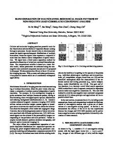
Fig. 1. Procedure for subtracting an extracted signal’s FFT from the source FFT

she splits each sound segment into 7 equal intervals. Because different instruments require different lengths, we use a new approach to look at the time it takes for the transient duration to reach the quasi-steady state of the fundamental frequency. It is estimated by computing the local cross-correlation function of the sound object, and the mean time to reach the maximum within each frame. The classifiers we built for training/testing are based on the following MPEG-7 descriptors: AudioSpectrumCentroid. It is a description of the center of gravity of the log-frequency power spectrum. Spectrum centroid is an economical description of the shape of the power spectrum. It indicates whether the power spectrum is dominated by low or high frequencies and, additionally, it is correlated with a major perceptual dimension of timbre; i.e.sharpness. To extract the spectrum centroid: 1. Calculate the power spectrum coefficients; 2. Power spectrum coefficients below 62.5 Hz are replaced by a single coefficient, with power equal to their sum and a nominal frequency of 31.25 Hz;3. Frequencies of all coefficients are scaled to an octave scale anchored at 1 kHz. AudioSpectrumSpread. It is a description of the spread of the log-frequency power spectrum. Spectrum spread is an economical descriptor of the shape of the power spectrum that indicates whether it is concentrated in the vicinity of its centroid, or else spread out over the spectrum. It allows differentiating between tone-like and noise-like sounds. To extract the spectrum Spread, we calculate the spectrum spread as the RMS deviation with respect to the centroid, on an octave scale.

7

HarmonicSpectralCentroid. It is computed as the average over the sound segment duration of the instantaneous HarmonicSpectralCentroid within a running window. The instantatneous HarmonicSpectralCentroid is computed as the amplitude (linear scale) weighted mean of the harmonic peaks of the spectrum. To extract the Harmonic Spectral Centroid, 1. Estimate the harmonic peaks over the sound segment. 2. Calculate the instantaneous HarmonicSpectralCentroid. 3. Calculate the average HarmonicSpectralCentroid for the sound segment. HarmonicSpectralDeviation. It is computed as the average over the sound segment duration of the instantaneous HarmonicSpectralDeviation within a running window which is computed as the spectral deviation of log-amplitude components from a global spectral envelope. The Harmonic Spectral Deviation is extracted using the following algorithm 1. Estimate the harmonic peaks over the sound segment. 2. Estimate the spectral envelope. 3. Calculate the instantaneous HarmonicSpectralDeviation. 4. Calculate the average HarmonicSpectralDeviation for the sound segment. HarmonicSpectralSpread. It is computed as the average over the sound segment duration of the instantaneous HarmonicSpectralSpread within a running window computed as the amplitude weighted standard deviation of the harmonic peaks of the spectrum, normalized by the instantaneous HarmonicSpectralCentroid. It is extracted using the following algorithm 1. Estimate the harmonic peaks over the sound segment. 2. Estimate the instantaneous HarmonicSpectralCentroid. 3. Calculate the instantaneous HarmonicSpectralSpread for each frame. 4. Calculate the average HarmonicSpectralSpread for each sound segment. HarmonicSpectralVariation. It is the mean over the sound segment duration of the instantaneous HarmonicSpectralVariation. The instantaneous HarmonicSpectralVariation is defined as the normalized correlation between the amplitude of the harmonic peaks of two adjacent frames. It is extracted using the following algorithm. 1. Estimate the harmonic peaks over the sound segment. 2. Calculate the instantaneous HarmonicSpectralVariation each frame. 3. Calculate the HarmonicSpectralVariation for the sound segment.

4

Experimental Procedures

In this research, we applied four different types of noise to built our testing dataset of 14 sounds described in Tables 1, 2. The second table represents randomly selected four of the resultant new sounds for testing. This testing consisted of binary classification of violin against a 25 varying pitches of a Steinway Piano taken from the MUM database. We used the remaining sounds in 3 for training. Essentially, we now had a training set that was void of any of the combination in the training set 4. In analyzing the results we found that the system correctly classified all the synthesized using four different classifiers. We did observe however that the original sound of violin from the MUMs database was incorrectly classified, without other original violin sounds from MUMs in the

8

training set, by three of the classifiers: Tree J48, Logistic Regression Model, and Bayesian Network. Thus, in this research, we conclude that the original sounds from MUMs and the synthesized sound, which were produced by our subtraction algorithm, can form a robust database, which can represent similar sounds of recordings from different sources. We consider the transient duration as the time to reach the quasi-steady state of fundamental frequency. Thus we only apply it to the harmonic descriptors, since in this duration the sound contains more timbre information than pitch information of the note, which is highly relevant to the fundamental frequency. The fundamental frequency is estimated by first computing the local cross-correlation function of the sound object, and then computing mean time to reach its maximum within each frame, and finally choosing the most frequently appearing resultant frequency in the quasi-steady status. In each frame i, the fundamental frequency is calculated in this form: f (i) =

Sr Ki /ni

(4)

where Sr is the sample Frequency, n is the total number of r(i, k)’s local valleys across zero, where k ∈ [1, Ki ]. See formula. Ki is estimated by k as the maximum fundamental period by the following formula, where r(i, k) reaches its maximum value. ω is the maximum fundamental period expected. ,v um+n−1 m+n−1 m+n−1 X X u X r(i, k) = s(j)s(j − k) t s(j − k)2 s(j)2 , k ∈ [1, Sr × ω] j=1

j=m

j=m

(5)

Table 5. Overall Accuracy Results Tree J8, Logistic, Local Weighted Learning, Bayesian Network . T reeJ48 Logistic LW L BayesianN etwork Accuracy 83.33%

83.33%

100% 83.33%

Table 6. Individual Results. T reeJ48 Logistic LW L BayesianN etwork 4C violin noise 01 02 04 4C violin noise 01 03 4C violin noise 01 04 4C violin noise 03 04 Subtracted Piano Sounds

Yes Yes Yes No Yes

Yes Yes Yes No Yes

Yes Yes Yes Yes Yes

Yes Yes Yes No Yes

9

5

Conclusion

Automatic sound indexing should allow labeling sound segments with instrument names. In our research, we start with the singular, homophonic sounds of musical instruments, and then extend our investigations to simultaneous sounds. This paper is focussing on the mix of two instruments sounds, the construction of successful classifiers for identifying them, and developing a new theory which we can easily extend to the mix of several sounds. Knowledge discovery techniques are applied at this stage of research. First of all, we discover rules that recognize various musical instruments. Next, we apply rules from the obtained set, one by one, to unknown sounds. By identifying so called supporting rules, we are able to point out which instrument is playing (or is dominating) in the given segment, and in what time moments this instrument starts and ends playing.

6

Acknowledgements

This research is supported by the National Science Foundation under grant IIS0414815.

References [1]

[2]

[3]

[4]

[5]

[6] [7]

[8]

Lewis R., Zhang X., Ras, Z.: ”A Knowledge Discovery Model of Identifying Musical Pitches and Instrumentations in Polyphonic Sounds.”, Special Issue, International Journal of Engineering Applications of Artificial Intelligence, 2007, will appear Herault J.,Jutten C.:”Space or time adaptive signal processing by neural network models.” American Institute of Physics Neural Networks for Computing. Vol. 151 Editor: J. S. Denker New York 3rd(1986)206–211 Bingham, E: ”Advances In Independent Component Analysis With Applications To Data Mining” Helsinki University of Technology: PhD Dissertation, Helsinki University of Technology. (2003) 07–11 Amari, S. et al: ”Multichannel blind deconvolution and equalization using the natural gradient” Proc. IEEE Workshop. , Signal Processing Advances in Wireless Comm. (1997) 101–104 Smaragdis, P. et al: ”Blind separation of convolved mixtures in the frequency domain” Proc. IEEE Workshop. , IEEE Procedures Neurocomputing: vol: 22 (1998) 21–34 Lambert, R. H and Bell A.J.: ”Blind separation of multiple speakers in a multipath environment”, IEEE Proc. ICASSP: April (1997) 423–426 Kostek, B.et al: ”Estimation of Musical Sound Separation Algorithm Effectiveness Employing Neural Networks” Journal of Intelligent Information Systems, SpringerHoughton Mifflin Company May, Vol:24 number 2/3 (2005) 133–135 Fujinaga, I and MacMillan, K: ”Realtime recognition of orchestral instruments” Proceedings of the International Computer Music Conference - Best Presentation Award, SpringerHoughton Mifflin Company (2000) 141–143

10 [9]

[10]

[11]

[12]

[13]

[14]

[15] [16]

[17] [18]

[19] [20] [21]

Eronen, A., Klapuri, A.: ”Musical Instrument Recognition Using Cepstral Coefficients and Temporal Features” In Proceedings of the IEEE International Conference on Acoustics, Speech and Signal Processing, ICASSP SpringerHoughton Mifflin Company(2000) 753–756 Zhang, T.: ”Instrument classification in polyphonic music based on timbre analysis” SPIE’s Conference on Internet Multimedia Management Systems II part of ITCom’01, Denver, Aug. 4519 (2001) 136– 147 Slezak, D., Synak, P., Wieczorkowska, A. and Wroblewski, J.: ”KDD-based approach to musical instrument sound recognition.” Hacid, M.S., Ras,Z.W., Zighed, D.A., Kodratoff Y. (eds.): Foundations of Intelligent Systems.Proc. of 13th Symposium ISMIS 2002, Lyon, Franc 4519 Berlin, Heidelberg Springer-Verlag (2002) 28– 36 Eronen, A.: ”Musical instrument recognition using ICA-based transform of features and discriminatively trained HMMs” In Proceedings of Processing and its Applications, ISSPA 2003, Paris, France, 1-4 July, Proceedings of the Seventh International Symposium on Signal Processing(2003) 133–136 Agostini. M, Longar M and Pollastri, E.: ”Musical Instrument Timbres Classification with Spectral Features” EURASIP Journal on Applied Signal Processing, volume issue 1 (2003)5–14 Kostek, B.: ”Musical Instrument Classification and Duet Analysis Employing Music Information Retrieval Techniques.” Proc. of the IEEE.92(4) (2004)712–729 Zweig, O.: ”Speech Recognition with Dynamic Bayesian Networks” Ph.D. dissertation, Univ. of California, Berkeley, CA. (1998) Livescu,K., Glass, J., and Bilmes, J.: ”Hidden Feature Models for Speech Recognition Using Dynamic Bayesian Network” Geneva, Switzerland Proc. Eurospeech September (2003) 2529-2532 Quinlan,J.: ”C4.5: Programs for Machine Learning” Morgan Kaufman, San Mateo CA (1993) Wieczorkowska, A.: ”Classification of musical instrument sounds using decision trees” 8th International Symposium on Sound Engineering and Mastering, ISSEM’99 (1999) 225– 230 le Cessie, S., and van Houwelingen, J.: ”Ridge Estimators in Logistic Regression” Applied Statistics, 41, no. 1 (1992)191–201 Atkeson C., Moore, A., and Schaal, S.: ”Locally Weighted Learning for Control” Artificial Intelligence Review, 11 no. 1-5 Feb. (1997) 11–73 Wieczorkowska A., et al.: ”Application of Temporal Descriptors to Musical Instrument Sound” Journal of Intelligent Information Systems, Integrating Artificial Intelligence and Database Technologies, volume 21, no. 1, July (2003)