IEEE TRANSACTIONS ON NEURAL NETWORKS, VOL. 16, NO. 3, MAY 2005
513
Neural Network Learning Algorithms for Tracking Minor Subspace in High-Dimensional Data Stream Da-Zheng Feng, Member, IEEE,, Wei-Xing Zheng, Senior Member, IEEE, and Ying Jia
Abstract—A novel random-gradient-based algorithm is developed for online tracking the minor component (MC) associated with the smallest eigenvalue of the autocorrelation matrix of the input vector sequence. The five available learning algorithms for tracking one MC are extended to those for tracking multiple MCs or the minor subspace (MS). In order to overcome the dynamical divergence properties of some available random-gradient-based algorithms, we propose a modification of the Oja-type algorithms, called OJAm, which can work satisfactorily. The averaging differential equation and the energy function associated with the OJAm are given. It is shown that the averaging differential equation will globally asymptotically converge to an invariance set. The corresponding energy or Lyapunov functions exhibit a unique global minimum attained if and only if its state matrices span the MS of the autocorrelation matrix of a vector data stream. The other stationary points are saddle (unstable) points. The globally convergence of OJAm is also studied. The OJAm provides an efficient online learning for tracking the MS. It can track an orthonormal basis of the MS while the other five available algorithms cannot track any orthonormal basis of the MS. The performances of the relative algorithms are shown via computer simulations. Index Terms—Convergence, eigenvalue decomposition (EVD), energy function, invariance set, learning algorithm, Lyapunov function, minor subspace (MS), neural network, stationary point, stability.
I. INTRODUCTION
T
HE MINOR subspace (MS) is a subspace spanned by all the eigenvectors associated with the minor eigenvalues of the autocorrelation matrix of a high-dimensional vector sequence. The MS that is also called the noise subspace (NS) has been extensively used in array signal processing [1], [2]. The NS tracking is a primary requirement in many real-time signal processing tasks such as the adaptive direction-of-arrival (DOA) estimation [3], and the data compression in data communications. In particular, the adaptive solution of a total least squares problem in adaptive signal processing [4], [5] requires to track the MS. In addition, the MS analysis is also an important feature extraction technique from a high-dimensional data sequence. For example, when the pattern separation is not achieved by using the principal components, some minor eigen components of a high-dimensional vector sequence may be the
Manuscript received June 5, 2003; revised February 20, 2004. This work was supported in part by the National Natural Science Foundation of China and in part by a research grant from the Australian Research Council. D.-Z. Feng is with the National Laboratory for Radar Signal Processing, Xidian University, 710071 Xi’an, P.R. China (e-mail:
[email protected]). W.-X. Zheng is with the School of QMMS, University of Western Sydney, Penrith South DC, NSW 1797, Australia (e-mail:
[email protected]). Y. Jia is with the Intel China Research Center, Beijing 100080, China (e-mail:
[email protected]). Digital Object Identifier 10.1109/TNN.2005.844854
key feature for pattern separation and recognition. Although the MS can be efficiently obtained by the algebraic approaches such as QR decomposition, such approaches usually have the per data update, where computational complexity and are the dimensions of the high-dimensional vector sequence and the MS, respectively. Hence, it is interesting to find some learning algorithms with lower computational complexity for adaptive signal processing applications. The adaptive algorithms for tracking one minor component (MC) have been proposed by several authors [6]–[11], all resulting in adaptive implementation of Pisarenko’s harmonic retrieve estimator [12]. Thompson [6] proposed an adaptive algorithm for extracting the smallest eigenvector from a high-dimensional vector stream. Yang and Kaveh [10] extended Thompson’s algorithm [6] to estimating multiple MC with the inflation procedure. However, Yang and Kaveh’s algorithm requires normalized operation. Oja [13], Xu et al. [14], and Wang and Karhunen [15] proposed several efficient algorithms that can avoid the normalized operation. Especially, the MC concept was first given in [14]. Luo et al. [16] presented a minor component analysis (MCA) algorithm that does not need any normalized operation. Recently, some good modifications for Oja’s MS-tracking algorithms have been proposed in [17]–[19]. Interestingly, Solo and Kong [20] carefully analyzed these algorithms. Moreover, the more realistic properties of these algorithms should be studied by the techniques used in [21]. In the recent decade, many algorithms [4], [11], [13]–[19], [22]–[26] for tracking the MS or MC have been proposed on the basis of the feedforward neural network models. Mathew and Reddy [11] proposed the MS algorithm based on a feedback neural network structure with a sigmoid activation function. Chiang and Chen [23] showed that a learning algorithm can extract multiple MCs in parallel with the appropriate initialization instead of the inflation method. On the basis of an information criterion and by extending and modifying the total least mean squares (TLMS) algorithm [4], Ouyang et al. [24] developed an adaptive MC tracker that automatically finds the MS without using the inflation method. Recently, Cirrincione et al. [18], [26] proposed the learning algorithm called MCA-EXIN that may have the satisfactory convergence. Zhang and Leung [25] proposed a much general model for the MC and provided an efficient technique for analyzing the convergence properties of these algorithms. The objective of the present paper is to find more satisfactory learning algorithms for adaptively tracking the MS. The paper is organized as follows. In Section II, some formulations relative to the MC and MS are given. We simply review some
1045-9227/$20.00 © 2005 IEEE
Authorized licensed use limited to: XIDIAN UNIVERSITY. Downloaded on August 14, 2009 at 08:17 from IEEE Xplore. Restrictions apply.
514
IEEE TRANSACTIONS ON NEURAL NETWORKS, VOL. 16, NO. 3, MAY 2005
available learning algorithms for tracking one MC, and propose a novel algorithm for tracking one MC. In Section III, some available and the proposed learning algorithms are extended for tracking the MS or the multiple MC, and their dynamical instability is further analyzed. Section IV carefully investigates the properties of the stationary points of the novel nonquadratic criteria associated with the proposed learning algorithm. In Section V, we study the globally asymptotic convergence of the averaging differential equation associated with the learning algorithm. In Section VI, computer simulation results are presented. Finally, we give some conclusions in Section VII.
it is easy to show that it is also possible that MCA EXIN converges to infinity [also see (3.18) and (3.19)]. Thus, the available learning algorithms for tracking the MC or MS seem to work unsatisfactorily. B. Algorithm An interesting algorithm is as follows: (2.1a) (2.1b)
II. NOVEL ALGORITHM FOR TRACKING ONE MC A. MS Let be an -dimensional zero-mean, Gaussian stationary, temporally white vector sequence with the posi. tive–definite autocorrelation matrix and denote the eigenvalues and Let the corresponding eigenvectors of , respectively. We shall such that arrange the orthonormal eigenvectors the corresponding eigenvalues are in a nondecreasing order: . The eigenvalue decomposition (EVD) of is represented as , and . where The eigenvectors associated with the smallest eigenvalues of the data vector are defined of the autocorrelation matrix is referred to as as the minor components (MC), and the number of the minor components [13], [14], [18], [26]. The eigenvectors associated with the smallest eigenvalue of of the data vector are called the autocorrelation matrix the smallest component. The subspace spanned by the minor components is called the MS. In some applications, we require where is the only to find the MS spanned by dimensions of the MS. In array processing [1], [2], it is usually assumed that the noise is spatially-temporally white. Then the eigenvalues associated only with the noise are smaller than the other eigenvalues associated with the signal. Usually, should be appropriately selected such that and . It is worth mentioning that linear neural nets are the simplest neurons to construct a neural network. Interestingly, a linear neuron trained by an unsupervised constrained Hebbian rule [13] can track the principal component from an input vector sequence. Similarly, a linear neuron trained by an unsupervised constrained anti-Hebbian rule [13]–[16] can adaptively extract the minor component from a multiple dimensional data stream. The available learning algorithms for tracking the MC or MS have careof the autocorrelation matrix fully analyzed in [18], [19], and [26], and simply referred to as algorithms OJAn, LUC, and FENG. It is possible that OJAn and LUC converge to infinity. In addition, the algorithm FENG seems to be simplest but it may work unsatisfactorily as pointed out in [18], [24], and [26]. Thus, a modified algorithm was given in [24] and is here called FENGm. Moreover, Cirrincione et al. developed the Rayleigh-quotient-based random gradient flow (called MCA EXIN [18], [26]) that has the good convergence. In fact, by using the analytical approach given in [19] and [26]
Since this leaning algorithm is very similar to the OJAn and can be considered as a modification of the OJAn, we refer to it as OJAm. Under certain assumptions [20], [21], [27], [28], the application of the stochastic approximation theories [20], [21], [27], [28] leads to the following averaging equation associated with (2.1):
(2.2) A cost or energy function of (2.2) is expressed by (2.3) Although (2.1) is very similar to the OJAn, is completely different from . It is easily shown that for any is finite. Moreover, difconstant the set with respect to by the chain rule along ferentiating the solution of (2.2) yields
(2.4) This shows that is a Lyapunov function [29]. Thus, (2.2) is globally asymptotically convergent. Now we show that (2.1) does not have the same effect as the sudden (dynamical) divergence in the OJAn, and LUC [18], [26]. It holds
Authorized licensed use limited to: XIDIAN UNIVERSITY. Downloaded on August 14, 2009 at 08:17 from IEEE Xplore. Restrictions apply.
(2.5)
FENG et al.: NEURAL NETWORK LEARNING ALGORITHMS FOR TRACKING MINOR SUBSPACE IN HIGH-DIMENSIONAL DATA STREAM
515
If the learning factor is small enough and the input vector is bounded, then we have
for for
(2.6)
This shows that tends to one if , which is called the one-tending property (OTP). along the solution of On the other hand, differentiating (2.2) yields
for for for
(2.7)
tends to one if This also shows that . with modulus one Remark 2.1: The OTP indicates that should be selected as the initial value of the OJAm. Otherwise, an inappropriate initial value may result in that the OJAm with a larger learning factor has some practical limitations similar to the basic Hebbian model [21]. Example 2.1: Since the LUC is easiest to diverge and the FENG is most seriously fluctuated as shown in [18] and [26], simulations are given for comparing the OJAn, MCA EXIN, FENGm [24], and OJAm only. Here, only the smallest component is extracted. The vector data sequence is generated by (2.8) is Gaussian, spawhere tially-temporally white and randomly produced. The learning factors in the OJAn, FENGm and OJAm are fixed at 0.2, while learning factor in the MCA EXIN is taken as 0.4. All the algorithms start from the same initial value that is randomly produced and normalized to modulus one. The evolutionary curves and the following index parameter: of (2.9) versus the iteration number are shown in Fig. 1(a) and (b). The obtained results illustrate that the OJAn has the faster divergent property, the MCA EXIN is slowly divergent, the FENGm is randomly fluctuated near a fixed positive constant, and the OJAm has the OTP. This shows that the OJAm for tracking one MC works more satisfactorily than the OJAn, MCA EXIN, and FENGm.
Fig. 1. (a) Denotes the evolution curves of the norm of the weight vector versus the iteration number, while (b) denotes the evolution curves of the index parameter versus the iteration number. This shows that the OJAn and the MCA EXIN are fast and slowly divergent, respectively, while the FENGm and OJAm are convergent.
An extended form of the OJAm for tracking MS is as foldenote the weight lows. Let matrix, where represents the th column vector of and also denotes the weight vector of the th neuron of a multiple-input–multiple-output (MIMO) linear neural network. The input–output relation of the MIMO linear neural network is described by (3.1) The extended learning algorithm for training the weight matrix is represented as
III. ALGORITHMS FOR TRACKING MS The learning algorithm given previously extracts only one minor component. In fact, this algorithm can easily be extended for tracking the multiple MC or MS.
(3.2) It should be noted that (3.2) is no trivial extension of the (2.1). Although (2.1) has many extended forms, they may be difficult
Authorized licensed use limited to: XIDIAN UNIVERSITY. Downloaded on August 14, 2009 at 08:17 from IEEE Xplore. Restrictions apply.
516
IEEE TRANSACTIONS ON NEURAL NETWORKS, VOL. 16, NO. 3, MAY 2005
to find the corresponding Lyapunov functions in order to analyze their stability. Under the similar conditions to those defined in [21], using the techniques of the stochastic approximation theory [27], [28] we can deduce the corresponding averaging differential equation
(3.3) The energy function associated with (3.3) is given by (3.4) The gradient of
with respect to
(3.11) Similarly, we can also give the averaging differential equations associated with the formulas (3.8)–(3.11) and the corresponding energy functions [31]. More importantly, the averaging equations associated with the formulas (3.8)–(3.10) have the common energy function. It can be shown that such energy function with an infinite invariance set is not the Lyapunov function [29]. Lemma 3.1: Given the weight matrix defined in (3.1) and (3.8)–(3.10), there exists the following orthogonality:
is given by [30] (3.12) (3.5)
Clearly, (3.3) is equivalent to the following equation: (3.6) Differentiating
Theorem 3.1 (Dynamical Instability): If the learning factor is not equal to zero, then the state flows in the learning algorithms OJAn, LUC, and MCA EXIN for tracking the MS are divergent. Proof: By using (3.8) and (3.12) inductively, we have
along the solution of (3.3) yields
(3.7) Since the extended form of the OJAm has the Lyapunov function only with a lower bound [29], the corresponding averaging equation converges to the common invariance set from any initial value . It is worth mentioning that since the deterministic discretetime formulation is basically different from the continuous-time equations [21], the global convergence of the deterministic discrete-time formulation associated with (3.2) should be carefully analyzed, which is pretty difficult. Thus, we should constrain the as and select the learning initial value factor small enough. Similarly, we can get nontrivial extended forms of the algorithms OJAn, LUC, MCA EXIN, and FENGm as follows. The extended learning algorithms associated with the algorithms OJAn [13], [14], LUC [16], MCA EXIN [18], [26], and FENGm [24] are, respectively, given by
(3.13) This shows that
(3.14) Moreover, since it usually holds (3.15) , for the OJAn, there is generally which shows that the state flow in (3.8) will increase infinitely. For the LUC, we have similarly
(3.16) Since there usually exists
(3.8) (3.17) (3.9)
for the random system LUC, we deduce that there is almost , which shows that the state flow in the learning algorithm LUC will increase infinitely. For the MCA EXIN, we have similarly
(3.10) Authorized licensed use limited to: XIDIAN UNIVERSITY. Downloaded on August 14, 2009 at 08:17 from IEEE Xplore. Restrictions apply.
(3.18)
FENG et al.: NEURAL NETWORK LEARNING ALGORITHMS FOR TRACKING MINOR SUBSPACE IN HIGH-DIMENSIONAL DATA STREAM
Since it usually holds
(3.19) for
the
random
system
MCA EXIN, we have , which shows that the state flow in the learning algorithm MCA EXIN will also increase infinitely. This completes the Proof of Theorem 3.1. Remark 3.2: Cirrincione et al. [26] refer to the infinite increase of the state flows in the OJAn and LUC as the sudden divergence. In fact, only several algorithms sometimes produce such a sudden divergence. Thus, we refer to the infinite increase of the state flows as the dynamical instability. The previous theorem shows that although the deterministic continuous-time formulation associated with the random algorithms (3.8), (3.9), and (3.10) may be stable, the random algorithms (3.8), (3.9), and (3.10) may still be dynamically unstable. is Theorem 3.2 (Boundedness): If the learning factor small enough and the input vector is bounded, then the state flows in the learning algorithms FENGm for tracking the MS are bounded. is small enough and Proof: Since the learning factor the input vector is bounded, we have
(3.20) for the FENGm. Notice that in the previous formula the secondorder terms associated with the learning factor have been neglected. It holds
(3.21) It is obviously seen that there exists a large enough such that , which results in . Thus, the state flow in the FENG is bounded. Theorem 3.3 (Boundedness): If the learning factor is small enough and the input vector is bounded, then the state flow in the learning algorithm OJAm for tracking the MS is bounded. Proof: It can be proved in a similar way to that proving Theorem 3.2. We will research elaborately the globally asymptotical convergence of only the algorithm OJAm in the next two sections. IV. LANDSCAPE OF NONQUADRATIC CRITERIA For convenience of analysis, first define as an permutation matrix in which each column has exactly one nonzero element equal to 1, and each row has, at most, one nonzero ele. Let and be the orthogonal ment, where
517
dimatrices, unless specified otherwise. Let be the . Let denote an inagonal matrix equal to has exactly teger number such that the permutation matrix the nonzero entry equal to 1 in row and column . Let be a associated with and . diagonal matrix Some important properties of the matrix operation can be found in [32]. in the domain Given , we study the following nonquadratic criterion (NQC) for tracking the MS: (4.1) Lemma 4.1: has a lower bound and approaches and . infinity from above as Note that Lemma 4.1 is clearly satisfied. Lemma 4.2: If is expanded by the eigenvector basis into (4.2) then we can find the NQC for the expanded coefficient matrix (4.3) is an expanded coefficient matrix. Clearly, where (4.5) represents an equivalent form of (4.1). is depicted by the following The landscape of two theorems. Since the matrix differential method will be used extensively in deriving derivatives, interested readers may refer to [30] for details. is a stationary point of in the Theorem 4.1: , where consist domain if and only if of the eigenvectors of . , in fact, defines a stationary set of Note that . Considering Lemma 4.2, we know that Theorem 4.1 is equivalent to the following Corollary 4.1. is a stationary point of in the Corollary 4.1: if and only if . domain Proof: See the Appendix. Similarly, notice that yields a stationary set of . Theorem 4.1 establishes the property of all the stationary . The next theorem further distinguishes points of spanning the MS the global minimum point set attained by from the other stationary points that are saddle (unstable) points. has a global minTheorem 4.2: In the domain imum that is attained when and only when , where . At a global minimum, . All the other stationary points are saddle (unstable) points of . By Lemma 4.2, again, it can be shown that Theorem 4.2 is equivalent to the following Corollary 4.2. has a global Corollary 4.2: In the domain minimum that is attained when and only when , where , where is an permutation matrix. . At a global minimum, we have are saddle All the other stationary points (unstable) points of . Proof: See the Appendix.
Authorized licensed use limited to: XIDIAN UNIVERSITY. Downloaded on August 14, 2009 at 08:17 from IEEE Xplore. Restrictions apply.
518
IEEE TRANSACTIONS ON NEURAL NETWORKS, VOL. 16, NO. 3, MAY 2005
It is easily shown that denotes a global minimum . point set of We make the following remarks. Remark 4.1: From the previous theorems, it is seen that the automatically orthonormalizes the minimum of columns of . Therefore, we need not impose any explicit orthogonal constrains on . Remark 4.2: At the minimum of only produces an arbitrary orthonormal basis of the MS but not the mulis an orthogonal projectiple MC. However, tion onto the MS and can be uniquely determined. has a global minimum set and no Remark 4.3: local ones. Thus, the iterative algorithms, like the gradient descent search algorithm for finding the global minimum point of , are guaranteed to globally converge to the desired MS for the proper initialization of in the domain (also see Section V). The presence of the saddle points does not cause any problems because they are avoided due to truncation error in practice computation. Furthermore, it should be noted that determine partly the difthe different landscapes of ferent convergence speed of their corresponding gradient search algorithms. V. GLOBAL ASYMPTOTICAL CONVERGENCE We now study the convergence properties of the OJAm alis the stagorithm by considering its gradient rule. When tionary processes and the learning factor is small enough, the discrete-time difference equation can be approximated by the corresponding continuous-time ordinary differential equation [13]–[15], [20], [21], [27], [28]. By analyzing the global convergence of this continuous-time ordinary differential equation, we can establish the conditions for the global convergence of the OJAm learning algorithm. By the Lyapunov function approach [29], we need to answer the following questions. 1) Is this dynamical system able to globally converge to the MS solution? 2) What is the domain of attraction around the equilibrium point attained at the MS, or equivalently, what is the initial condition to ensure the global convergence? These questions are answered by the next theorem. Theorem 5.1: Given the ordinary differential equation (3.3) , then globally asymptotand the initial value as , ically converges to a point in the set and denotes an unitary where orthogonal matrix. globally asymptotiProof: From (3.6) we know that cally converges to a point in the invariance (stationary point) set . Since at a saddle (unstable) point (3.3) is unstable, of globally asymptotically converges to a point in the global minimum point set . This completes the Proof of Theorem 5.1. VI. COMPUTER SIMULATIONS Since the LUC is easiest to diverge [26], the FENG is most seriously fluctuated [26], and the learning factors in the LUC
and FENG are difficult to be selected appropriately, computer simulations are conducted only for comparing the OJAn, MCA EXIN, FENGm and OJAm for tracking the MS. Here, an MS with dimension 5 is tracked. The vector data sequence is generated by (6.1) where is randomly produced. Deviation of a state matrix from the orthogonality is defined as
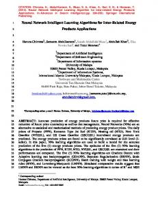
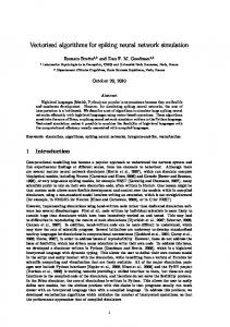
(6.2) The norm of a state matrix is given by (6.3) Example 6.1: Let , and be Gaussian, spatially-temporally white, and randomly produced. We simulate the algorithms starting from the same which is randomly produced. The learning initial value factors in the OJAn, MCA EXIN, FENGm, and OJAm are taken as 0.04, 0.4, 0.04, and 0.04, respectively. In the case with the , Fig. 2(a) and (b) shows the deviorthonormalization of ation and the index parameter versus the iteration number, respectively. , and Example 6.2: Let be Gaussian, spatially-temporally white and randomly produced. The learning factors in the OJAn, MCA EXIN, FENGm, and OJAm are taken as 0.08, 0.8, 0.08, and 0.08, respectively. In the similar cases to Example 6.1, we can get the results as shown in Fig. 3. The obtained simulation results show that the state matrices in the OJAn, MCA EXIN, and FENGm will not converge to an orthonormal basis of the MS, while the state matrix in the OJAm will tend to an orthonormal basis of the MS. Moreover, the norm of the state matrix of the OJAn fast increases, while the norm of the state matrix of the MCA EXIN, FENGm slowly increase. Thus, the OJAm seems to work more satisfactorily. VII. CONCLUSION This paper has developed an interesting modification of the Oja-type algorithms, called OJAm, which can work satisfactorily. Unlike some available random-gradient-based algorithms, the OJAm has no dynamical divergence property. The five available learning algorithms for tracking one minor component have been extended to those for tracking the multiple MC or MS. The averaging equation of the OJAm exhibits a single global minimum that is attainable if and only if its state matrix spans the MS of the autocorrelation matrix of a vector data stream. The other stationary points of the OJAm are saddle (unstable) points. We have studied the globally asymptotic stability of the averaging equation of the OJAm. The simulations have shown that most of the available random-gradient-based algorithms for tracking the MS converge to the MS at the same order of convergence speed, but the OJAm makes the corresponding state matrix tend to a column-orthonormal basis of the MS.
Authorized licensed use limited to: XIDIAN UNIVERSITY. Downloaded on August 14, 2009 at 08:17 from IEEE Xplore. Restrictions apply.
FENG et al.: NEURAL NETWORK LEARNING ALGORITHMS FOR TRACKING MINOR SUBSPACE IN HIGH-DIMENSIONAL DATA STREAM
Fig. 2. Here, the dimensions of the input vector sequence are 11 and the initial weight matrix is orthonromalized. (a) and (b) denote the evolution curves of the norm of state matrix, and deviation of the state matrix from the orthogonality versus the iteration number, respectively.
Since dient of [30]
Fig. 3. Here, the dimensions of the input vector sequence are 31 and the initial weight matrix is othonromalized. (a) and (b) denote the evolution curves of the norm of state matrix, and the deviation of the state matrix from the orthogonality versus the iteration number, respectively.
Conversely,
APPENDIX I PROOF OF COROLLARY 4.1 is positive–definite, it is invertible. The grawith respect to exists and is given by
519
at a stationary point should satisfy , which yields (A.3)
Premultiplying both sides of (A.3) by
, we obtain (A.4)
(A.1) Given
a point for any uniatry orthonormal by using Lemma 2.2, we have
in and
which implies that the columns of orthonormal at a stationary point of (A.4) we have
are column. From (A.3) and (A.5)
, where is a row Let that is an symmetric posivector, and take tive–definite matrix. Then the alternative form of (A.5) is (A.2) Authorized licensed use limited to: XIDIAN UNIVERSITY. Downloaded on August 14, 2009 at 08:17 from IEEE Xplore. Restrictions apply.
(A.6)
520
IEEE TRANSACTIONS ON NEURAL NETWORKS, VOL. 16, NO. 3, MAY 2005
Obviously, (A.6) shows the EVD for . Since is an symmetric positive–definite matrix, it has only the orthonormal has only the orleft-row eigenvectors, which shows that thonormal row vectors. Moreover, all the nonzero row vectors in form an orthonormal matrix, which shows that can always be represented as (A.7)
Since (B.6a) (B.6b) (B.5) becomes (B.7)
This completes the Proof of Corollary 4.1. APPENDIX II PROOF OF COROLLARY 4.2 has only a lower bound, and will apObviously, and . proach infinity from above as Thus, the global minimum is attained only by a stationary point . Like the method in [24], we can obtain the preof vious result through analyzing the Hessian matrices at all the stationary points. However, due to the complexity of the Hessian matrix, the method in [24] may not be easily applicable. in the stationary point By computing the values of set for the domain , we can directly verify is attained when and only that a global minimum of when (B.1) where the first row vectors of the permutation contain all the nonzero elements of the permutation . By substituting (B.1) into (4.3) and performing some algebraic operations, we can get as follows: the global minimum of
and which shows that the set not a global minimum point set. , we can always select a column As from such that
(B.8) . Moreover, we can always select a column from , so that
otherwise
(B.9) . Let have only the nonzero eleotherwise and have only the nonzero entry ment in row in row . Obviously, and , oth. Define an orthonormal matrix as erwise , where is a positive infinitesimal. Considering that and have one nonzero entry, this shows that
(B.10) Considering (B.6), (B.9), and (B.10), we have
(B.2) Moreover, we can determine whether a stationary point of is saddle (unstable) in such a way that within an infinitesimal neighborhood near the stationary point, there such that its value is less than is a point . . There exists, at least, a nonzero element in Let to for . Since and are the row vectors from two permutation matrices, there are certainly the two diagonal and matrices and such that . This yields (B.3a) (B.3b)
is
(B.11) Since
is an
permutation matrix, we can deduce (B.12)
Let
(B.13) Since matrix. Thus, we deduce that
is a positive–semidefinite
Thus, we have (B.14)
(B.4a) (B.4b) If and
for
are rearranged in a nondecreasing order , then there are , . This shows (B.5)
This shows that and is a saddle (unstable) point set. This completes the Proof of Corollary 4.2.
ACKNOWLEDGMENT The authors would like to thank the Associate Editor and the anonymous reviewers for their valuable comments and suggestions that have significantly improved the manuscript.
Authorized licensed use limited to: XIDIAN UNIVERSITY. Downloaded on August 14, 2009 at 08:17 from IEEE Xplore. Restrictions apply.
FENG et al.: NEURAL NETWORK LEARNING ALGORITHMS FOR TRACKING MINOR SUBSPACE IN HIGH-DIMENSIONAL DATA STREAM
REFERENCES [1] R. Schmidt, “Multiple emitter location and signal parameter estimation,” IEEE Trans. Antennas Propaga., vol. AP-34, no. 3, pp. 276–280, Mar. 1986. [2] K. Kumaresan and D. W. Tufts, “Estimating the angles of arrival of multiple plane waves,” IEEE Trans. Aerosp. Electron. Syst., vol. AES-19, no. 1, pp. 134–139, Feb. 1983. [3] T. S. Durrani and K. C. Shatman, “Eigenfilter approaches to adaptive array processing,” Proc. Inst. Elect. Eng. F, vol. 130, Feb. 1983. [4] D. Z. Feng, Z. Bao, and L. C. Jiao, “Total least mean squares algorithm,” IEEE Trans. Signal Process., vol. 46, no. 6, pp. 2122–2130, Aug. 1998. [5] C. E. Davila, “An efficient recursive total least squares algorithm for FIR adaptive filtering,” IEEE Trans. Signal Process., vol. 42, no. 2, pp. 268–280, Feb. 1994. [6] P. A. Thompson, “An adaptive spectral analysis technique for unbiased estimation in the presence of white noise,” in Proc. 13th Asilomar Conf. Circuits, Systems Computation, Pacific Grove, CA, 1979, pp. 529–533. [7] V. U. Reddy, B. Egardt, and T. Kailath, “Least squares type algorithm for adaptive implementation of Pisarenko’s harmonic retrieval method,” IEEE Trans. Acoust., Speech, Signal Process., vol. ASSP-30, no. 3, pp. 399–405, Jun. 1982. [8] J.-F. Yang, H.-T. Wu, and F.-K. Chen, “Simplified adaptive noise subspace algorithms for robust direction tracking,” Proc. Inst. Elect. Eng. F: Radar and Signal Processing, vol. 140, no. 5, pp. 329–334, Oct. 1993. [9] D. R. Fuhrmann and B. Liu, “Rotational search methods for adaptive Pisarenko harmonic retrieval,” IEEE Trans. Acoust., Speech, Signal Process., vol. ASSP-34, no. 6, pp. 1550–1565, Dec. 1986. [10] J.-F. Yang and M. Kaveh, “Adaptive eigensubspace algorithms for direction or frequency estimation and tracking,” IEEE Trans. Acoust., Speech, Signal Process., vol. ASSP-36, no. 2, pp. 241–251, Feb. 1988. [11] G. Mathew and V. U. Reddy, “Orthogonal eigensubspace estimation using neural networks,” IEEE Trans. Signal Process., vol. 42, no. 7, pp. 1803–1811, Jul. 1994. [12] V. F. Pisarenko, “The retrieval of harmonics from a covariance function,” Geophys. J. R. Astron. Soc., vol. 33, pp. 374–366, 1973. [13] E. Oja, “Principal component, minor component and linear neural networks,” Neural Netw., vol. 5, no. 6, pp. 927–935, 1992. [14] L. Xu, E. Oja, and C. Y. Suen, “Modified Hebbian learning for curve and surface fitting,” Neural Netw., vol. 5, no. 3, pp. 441–457, 1992. [15] L. Wang and J. Karhunen, “A unified neural bigradient algorithm for robust PCA and MCA,” Int. J. Neural Syst., vol. 7, pp. 43–67, 1996. [16] F. L. Luo and R. Unbehauen, “A minor subspace analysis algorithm,” IEEE Trans. Neural Netw., vol. 8, no. 5, pp. 1149–1155, Sep. 1997. [17] S. C. Douglas, S. Y. Kung, and S. Amari, “A self-stabilized minor subspace rule,” IEEE Signal Process. Lett., vol. 5, no. 12, pp. 328–330, Dec. 1998. [18] G. Cirrincione and M. Cirrincione, “Neural minor component analysis and TLS,” in Total Least Squares and Error-in-Variables Modeling: Analysis, Algorithms and Applications, S. van Huffel and P. Lemmerling, Eds. Norwell, MA: Kluwer, 2002, pp. 235–251. [19] A. Taleb and G. Cirrincione, “Against the convergence of the minor component analysis neurons,” IEEE Trans. Neural Netw., vol. 10, no. 1, pp. 207–210, Jan. 1999. [20] V. Solo and X. Kong, “Performance analysis of adaptive eigenanalysis algorithms,” IEEE Trans. Signal Process., vol. 46, no. 3, pp. 636–646, Mar. 1996. [21] P. J. Zufiria, “On the discrete-time dynamics of the basic Hebbian neuralnetwork node,” IEEE Trans. Neural Netw., vol. 13, no. 6, pp. 1342–1352, Nov. 2002. [22] G. Mathew, V. U. Reddy, and S. Dasgupta, “Adaptive estimation of eigensubspace,” IEEE Trans. Signal Process., vol. 43, no. 2, pp. 401–411, Feb. 1995. [23] C. T. Chiang and Y. H. Chen, “On the inflation method in adaptive noisesubspace estimator,” IEEE Trans. Signal Process., vol. 47, no. 4, pp. 1125–1129, Apr. 1999. [24] S. Ouyang, Z. Bao, G. S. Liao, and P. C. Ching, “Adaptive minor component extraction with modular structure,” IEEE Trans. Signal Process., vol. 49, no. 9, pp. 2127–2137, Sep. 2001. [25] Q. Zhang and Y.-W. Leung, “A class of learning algorithms for principal component analysis and minor component analysis,” IEEE Trans. Neural Netw., vol. 11, no. 2, pp. 529–533, Mar. 2000. [26] G. Cirrincione, M. Cirrincione, J. Herault, and S. Van Huffel, “The MCA EXIN neuron for the minor component analysis,” IEEE Trans. Neural Netw., vol. 13, no. 1, pp. 160–187, Jan. 2002.
521
[27] H. J. Kushner and D. S. Clark, Stochastic Approximation Methods for Constrained and Unconstrained Systems. New York: Springer-Verlag, 1976. [28] L. Ljung, “Analysis of recursive stochastic algorithms,” IEEE Trans. Automat. Contr., vol. AC-22, no. 4, pp. 551–575, Aug. 1977. [29] J. P. LaSalle, The Stability of Dynamical Systems. Philadelphia, PA: SIAM, 1976. [30] J. R. Magnus and H. Neudecker, Matrix Differential Calculus with Applications in Statistics and Econometrics, 2nd ed. New York: Wiley, 1991. [31] J. J. Hopfield, “Neural networks and physical systems with emergent collective computational abilities,” Proc. Nat. Acad. Sci. USA, vol. 79, pp. 2554–2558, 1962. [32] G. H. Golub and C. F. van Loan, Matrix Computations, 2nd ed. Baltimore, MD: The Johns Hopkins Univ. Press, 1989. Da-Zheng Feng (M’02) was born in December 1959. He received the B.Sc. degree from Xi’an University of Technology, Xi’an, China, in 1982, the M.S. degree from Xi’an Jiaotong University, Xi’an, China, in 1986, and the Ph.D. degree in electronic engineering from Xidian University, Xi’an, China, in 1995. From 1996 to 1998, he was a Postdoctoral Research Affiliate and an Associate Professor at Xi’an Jiaotong University. From 1998 to 2000, he was an Associate Professor at Xidian University. Since 2000, he has been a Professor at Xidian University. He has published more than 40 journal papers. His research interests include signal processing, intelligence information processing, and InSAR. Wei Xing Zheng (M’93–SM’98) was born in Nanjing, China. He received the B.Sc. degree in applied mathematics and the M.Sc. and Ph.D. degrees in engineering, in 1982, 1984, and 1989, respectively, all from the Southeast University, Nanjing, China. From 1984 to 1991, he was with the Institute of Automation, Southeast University, first as a Lecturer and later as an Associate Professor. From 1991 to 1994, he was a Research Fellow with the Department of Electrical and Electronic Engineering, Imperial College of Science, Technology, and Medicine, University of London, London, U.K.; with the Department of Mathematics, University of Western Australia, Perth, Australia; and with the Australian Telecommunications Research Institute, Curtin University of Technology, Perth. In 1994, he joined the University of Western Sydney, Sydney, Australia, where he has been an Associate Professor since 2001. He has also held various visiting positions in the Institute for Network Theory and Circuit Design, Munich University of Technology, Munich, Germany; with the Department of Electrical Engineering, University of Virginia, Charlottesville; and with the Department of Electrical and Computer Engineering, University of California, Davis. His research interests are in the areas of systems and controls, signal processing, and communications. He coauthored the book Linear Multivariable Systems: Theory and Design (Nanjing, China: Southeast Univ. Press, 1991). Dr. Zheng received the Chinese National Natural Science Prize awarded by the Chinese Government in 1991. He has served on the technical program committee of several conferences including the 34th IEEE International Symposium on Circuits and Systems (ISCAS 2001), the 41st IEEE Conference on Decision and Control (CDC 2002), and the 43rd IEEE Conference on Decision and Control (CDC 2004). He has also served on several technical committees, including the IEEE Circuits and Systems Society s Technical Committee on Digital Signal Processing (since 2001) and the IFAC Technical Committee on Modeling, Identification, and Signal Processing (since 1999). He served as an Associate Editor of the IEEE TRANSACTIONS ON CIRCUITS AND SYSTEMS I, from 2002 to 2004. He has been an Associate Editor of the IEEE Control Systems Society s Conference Editorial Board since 2000 and an Associate Editor of the IEEE TRANSACTIONS ON AUTOMATIC CONTROL since 2005. Ying Jia was born on July 24, 1971 in Xinjiang, China. He received the Ph.D. degree from the Institute of Acoustics, Chinese Academy of Science (CAS), Beijing, China, in 1999, and the M.S. and B.S. degrees from Xi’dian University, Xi’an, China, in 1996 and 1993, respectively. Since 1999, he has been a Senior Staff Researcher in Corporate Technology Group, Intel China Research Center, Beijing, China. His research interests include array signal processing, its applications in microphone array, wireless communication, audio and video signal processing, speech recognition and human–computer interface.
Authorized licensed use limited to: XIDIAN UNIVERSITY. Downloaded on August 14, 2009 at 08:17 from IEEE Xplore. Restrictions apply.