SIMULINK BLOCKSET FOR NEURO-FUZZY PREDICTIVE CONTROL Cristian Olaru, George Dragnea and Octavian Pastravanu Department of Automatic Control and Industrial Informatics, Faculty of Automatic Control and Computer Science Technical University “Gh. Asachi” of Iasi, Blvd. Mangeron 53A, 700050, Iasi, Romania Phone / Fax: +40-232-230751, E-mail:
[email protected]
Abstract: The paper presents a Simulink blockset that extends the usage of Simulink environment toward the area of neuro-fuzzy predictive control of non-linear processes. The blockset provides tools for identification, simulation and controller design based on neuro-fuzzy models. The user can circumvent the need for writing program codes, by simply operating with diagram blocks, in full accordance with the "drag and drop" technique specific to Simulink. The newly created blocks are easy to handle and versatile, permitting the selection of various options for model construction and control strategy. The first part of the article gives details about the algorithmic support and the software implementation. The second part illustrates the exploitation of the blocks for an example of reference tracking control taken from literature. Keywords: non-linear predictive control, neuro-fuzzy identification, neuro-fuzzy control, ANFIS procedure, Simulink.
1. INTRODUCTION The Model Based Predictive Control (MBPC) is a strategy that finds a control trajectory over a future time horizon based on a dynamic model of the process. In the last decades, MBPC has become an important and a distinctive part of control theory and has been widely used in the area of industrial applications. All predictive controllers are based on the fact that the process output can be predicted over a time horizon by using the past process inputs and outputs, if a suitable model of the plant is known. There are many algorithms proposed in literature for implementing a predictive control, such as: Model Algorithmic Control – MAC (Mehra and Rouhani, 1982), Extended Prediction Self - Adaptive Control – EPSAC (De Keyser and Van Cauwenberghe, 1985), Generalized Predictive Control – GPC (Clarke et el., 1992) and Unified Predictive Control – UPC (Kadirkamanathan, 1996). The mentioned algorithms are quite similar in the sense that they are based on
the same general ideas: receding horizon principle, plant model as part of the controller, prediction of the system output and optimization of a cost function. The differences between the algorithms consist in the used plant models and the chosen cost function. The model used in the predictive controller plays a decisive role in obtaining a successful control strategy that can be applied to a real plant. The model must be capable to accurately describe the process dynamics, it should be easy to implement and at the same time fast in simulation. Considering these points of view, for many plants, a neuro-fuzzy system can prove to be a good model to use in a predictive controller. This paper is dedicated to the efficient exploitation of the well-known environment MATLAB-Simulink for designing and testing neuro-fuzzy predictive controllers. It presents a Simulink blockset developed at the Department of Automatic Control and
Industrial Informatics of the Technical University "Gh. Asachi" of Iasi, that covers the standard problems of MBPC relying on neuro-fuzzy models. We have developed a blockset similar to the one developed in (Kloetzer and Pastravanu, 2004), except this new one is based on neuro-fuzzy techniques - the mathematical model is obtained with the ANFIS procedure (Jang, 1995). This blockset allows the user to operate only with block diagrams for model construction and validation, as well as for the simulation of predictive control strategies. Thus, the user can focus on the control engineering aspects of the application, by eliminating programming tasks, which are important time-consumers in the absence of such predesigned software modules. These modules are organized as a library of S-functions, fully compatible with the drag and drop philosophy of the Simulink package. In the construction of the current paper we incorporate the software facilities created by our previous work (Dragnea and Olaru, 2004) for identification and simulation experiments under Simulink, relying on neuro-fuzzy models. We also derive a full benefit from the experience accumulated by our research group (Kloetzer, et. al., 2001, Kloetzer and Pastravanu, 2004) in the exploitation of the MATLAB-Simulink environment for neuralnetwork-based identification and control of nonlinear dynamical systems. The paper is organized as follows: the first part presents the theoretical preliminaries of neuro-fuzzy predictive control (Section II), continuing with the presentation of the new Simulink library created for neuro-fuzzy system-based control applications (Section III), followed by a case study that illustrates the usage of the blocks in Section IV and finally, in Section V, some conclusions are formulated to underline the importance of the results. 2. PREDICTIVE CONTROL BASED ON NEURO-FUZZY MODELS An intuitive graphical representation of the predictive control strategy is given in Fig. 1. At each time moment k·T, where T is the sample time and it will be omitted in the following formulas for simplicity, the future control policy u is computed in the idea that the process output y will accurately follow the reference trajectory r. In presenting the basics of the standard predictive control, the following notations will be used: Nu – the control horizon; N1 – the minimum prediction horizon; N2 – the prediction horizon; λ – the weight factor; r – the reference trajectory. The predictive control based on neuro-fuzzy models uses a neuro-fuzzy system to calculate the future plant output and a cost function based on the error between the predicted process output and the reference trajectory. The cost function, which may be
different from case to case, is minimized in order to obtain the optimal input control that is applied to the non-linear plant. A possible form of the cost function, used in most predictive control algorithms, is given by the following expression: N2 2 J = ∑ [ r (k + i ) − y (k + i)] + i = N1 Nu 2 λ ∑ [u (k + i − 1) − u (k + i − 2)] i =1
(1)
Usually, the weight factor is considered λ = 0 and the minimum prediction horizon is N1 = 1. At each time moment k, the cost function J is minimized with respect to the vector containing the future input values: u = [u ( k + 1), u ( k + 2), ..., u (k + Nu )]T (2)
Fig. 1. MBPC strategy The process to be controlled is described by:
y ( k )= f ( y ( k−1),..., y ( k−n ), u ( k−d ),..., u ( k−d −m])),
(3) k , m, n, d ∈ N n+ m+1 → R is a smooth non-linear where f : R mapping describing the input-output transfer of a static system. The identification experiment can be organized according to a series-parallel scheme (Narendra and Parthasarathy, 1990). The following notations will be used to designate the future inputs and outputs of the neuro-fuzzy model: u (k + 1 − d ) = = [ u(k + 1 − d ), u(k + 1 − d − 1),..., u(k + 1 − d − m)]T (4) y(k + i − 1) = = [ y(k + i − 1), y(k + i − 2),..., y(k + 1 − n)]T
where i = N1...N2 denotes the order of the predictor, m and n are the number of delays for input and output of the model respectively, d is the dead time from (3) and k is the current time moment. By feeding the neuro-fuzzy system with the vectors from (4), one can obtain the ith - step ahead predictor y(k+i), as presented in Fig. 2. In computing the future outputs of the process, if N2 > Nu+d, after the (Nu + d)-th iteration, the control signal will be kept constant at a value equal to
u(k+Nu). The predictive control algorithm relies on steps described below for an arbitrary discrete-time instant k: • the previous iteration, after the minimization procedure at the moment k-1, has given the command vector u old = [u (k ), u (k + 1), ..., u (k + N u − 1)]T ; • the step ahead predictors y(k+i) of orders i=N1...N2, are calculated by using the vectors u(k+id), y(k+i-1); • the optimal control signal is achieved by minimizing the cost function J in (1) with respect to the command vector: u new = [u (k + 1), u (k + 2),...
classical manner. The blocks available in this library are presented in a compact form by fig.4. The NF_IDN (Fuzzy Training) block serves in constructing neuro-fuzzy model, whereas the NF_SIM (Fuzzy Simulator) block serves in simulating the model. Details on the implementation and exploitation of these blocks can be found in a previous work of ours (Dragnea and Olaru, 2004). The NF_CON (Neuro-fuzzy predictive controller) block is the latest created and added to the Simulink blockset presented in Fig. 4.
..., u (k + N u )]T .
Fig. 2. Computational strategy for neuro-fuzzy predictors. At the k-th time moment, the control signal u(k) is applied to the process and the algorithm is reiterated. At the first iteration, the initial input u(0) must be provided by the user. Considering the basic theoretical preliminaries of MPBC presented in this section, a block diagram of a standard predictive controller is depicted in Fig. 3.
Fig. 4. Components of the Simulink blockset developed for neuro-fuzzy-system-based control applications. The modular architecture of the NF_CON block is presented in Fig. 5. The nucleous of the controller is the predctrl, which treats the first and the third steps of the algorithm described in section 2. The procedure cost.m provides the computations requested by the second step of the algorithm and for the construction of the objective (cost) function J. This procedure is called from the main routine after the first step, and the returned objective function is minimized in the third step. For the minimization of the cost function, the procedure fmincon from the Optimal Toolbox was used, which allows imposing constraints for the values of the control input. At each iteration, the S-function predctrl stores a vector containing the last Nu values of the control signal applied to the plant and, at the next time moment, this vector will be used as an initial guess for starting the minimization.
Fig. 3. Basic structure of MBPC 3. BLOCKS AVAILABLE IN THE NEW LIBRARY AND THEIR USAGE The Simulink library dedicated to neuro-fuzzysystems-based control applications brings many advantages, as it offers a more attractive perspective for control engineering than writing codes in a
Fig. 5. Modular architecture of NF_CON block
the model was incorporated within the structure of the predictive controller via the NF_CON block. The Simulink diagram used for the closed-loop tests of the neuro-fuzzy predictive controller is presented in Fig. 7. The parameters required by the control algorithm (minimum prediction horizon N1 = 1, prediction horizon N2 = 3, control horizon Nu = 2, weight factor λ = 0 and initial input uinit = 0) were set by means of the dialog box of the NF_CON block.
Fig. 7. Simulink diagram used for testing the predictive control of the considered plant
Fig. 6. Dialog box for NF_CON block The dialog box of the NF_CON block, as you can see in Fig. 6, allows the user to specify the parameters related both to the neuro-fuzzy architecture (parameter vector, dead time, number of input and output delays in model (2)) and to the control algorithm (minimum prediction horizon, prediction horizon, control horizon, constraints for the control signal, weight vector and initial input). The reference trajectory must be stored in a workspace vector, because it is supposed to be a priori known. The vector containing the neuro-fuzzy model parameters has the same structure as the vector resulting from the identification with the Simulink block NF_IDN.
a.
4. ILLUSTRATIVE CASE STUDY In order to illustrate the usage of our Simulink blockset, this section presents the steps taken for the synthesis of a neuro-fuzzy predictive controller corresponding to the non-linear plant described by the difference equation (Liu et al., 1996): y (k ) =
2.5 y (k − 1) y (k − 2) + 1 + y 2 (k − 1) + y 2 (k − 2)
b. (5)
+0.3cos(0.5( y (k − 1) + y (k − 2)) + 1.2u (k − 1) Initially, the plant described by (5) was identified by using the NF_IDN block, with a sampling period T = 1 second. Then, the neuro-fuzzy model was validated by simulation, using the specific block NF_SIM. Generally speaking, these two steps must be reiterated (with different training parameters) until the obtained model exhibit a desired quality. Finally,
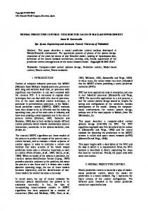
Fig. 8. Comparative plots of the controlled plant output (dashed line) and of the reference trajectory (full line) in case on unconstrained control action: a. piecewise linear reference signal; b. sinusoidal reference trajectory. Fig. 8 reproduces the results of a test when a neurofuzzy model was used by the predictive controller. Both figures prove a good tracking of the reference trajectory.
a.
a.
b. Fig. 9. Plot of the control action in case of: a. piecewise linear reference signal; b. sinusoidal reference trajectory.
b. Fig. 11. Plot of the constrained control action (-0.3; 0.3) in case of piecewise linear reference signal (a) and of the constrained control action (-0.4; 0.4) in case of sinusoidal trajectory. In case of high values for the amplitude or constraints for the control action the results are not satisfactory as the output cannot follow the reference in the lowfrequency area, as presented in Fig. 10.
a.
In this case study, when a neuro-fuzzy model is used, the results obtained by the predictive controller, are comparable with the results obtained in case of neural models (e.g. Kloetzer and Pastravanu, 2004), but the first one has a slight advantage as it is more complex than the neural model. Thus it can capture certain nonlinearities, which cannot be observed by the neural model. 5. CONCLUSIONS
b. Fig. 10. Comparative plots of the controlled plant output (dashed line) and reference trajectory (full line) in case of constrained control action (-0.3;0.3) for a piecewise linear reference signal (a) and in case of constrained control action (-0.4;0.4) for a sinusoidal reference trajectory (b).
We have developed a Simulink library that provides tools for identification, simulation and controller design based on neuro-fuzzy models. The exploitation of these tools is fully compatible with the "drag and drop" technique specific to Simulink and allows the user to focus on the Control Engineering problems, by getting rid of the traditional programming tasks. The newly created blocks are easy to handle and versatile, permitting the selection of various options for the model construction and the control strategy. The implementation of the blocks relies on functions available in MATLAB and its toolboxes, fact which ensures the robustness of the software.
The considered case study proves the utility of the Simulink blockset in developing accurate neurofuzzy models that can be successfully incorporated within predictive control schemes.
Acknowledgements: The first two authors are grateful to Mr. Marius Kloetzer for the generosity of sharing his experience in MATLAB-Simulink programming. REFERENCES Clarke, D.W., Mothadi, C. and Tuffs, P.S., (1987), “Generalized predictive control. Part I – The basic algorithm and Part II – Extensions and interpretations”, Automatica, vol. 23, pp. 137 – 160. De Keyser, R and Van Cauwenberghe, A.R.,(1985), “Extended prediction self – adaptive control”, IFAC Symposium on Identification and System Parameter Estimation, York, UK, pp. 1317 – 1322. Dragnea, G. , Olaru, C., Kloetzer, M. , Pastravanu, O., (2004), “Simulink tools for neuro-fuzzy based identification”, Symposium on Automatic Control and Computer Science, Iasi. Jang, J-S, “Neuro-Fuzzy Modelling and Control”, Proceedings of IEEE, 1995, 83, 3, 378 – 405.
Kloetzer, M., Ardelean, D. and Păstrăvanu, O., (2001), “Developing Simulink tools for teaching neural-net-based identification”, Med’01: The 9th Mediterranean Conference on Control and Automation, pp. 63 (abstract), paper on CDROM. Kloetzer, M. and Pastravanu O., (2004), “Simulink blockset for neural predictive control”, Transactions on Automatic Control and Computer Science, Vol. 49 (63), ISSN 1224600X Liu, G. P., Kadirkamanathan, V. and Billings S.A.,(1996), “Stable sequential identification of continuous nonlinear dynamical systems by growing RBF networks”, International Journal of Control, vol. 65, pp. 53 – 60. Mehra, R. K. and Rouhani, R., (1982), “Model algorithm control: review and recent development”, Proc. Engn. Foundation Conf. on Chemical Process Control II, Sea Island, Georgia, pp. 287 – 310. Narendra , K. S. and Parthasarathy, K., (1990), “Identification and control of dynamical systems using neural networks”, IEEE Transactions on Neural Networks, vol. 1, pp. 4 – 27. Soeterboek, R., (1992), Predictive Control. A Unified Approach, Englewood Cliffs, Prentice Hall, New York.