Neural Networks and Rational L Ã ukasiewicz Logic Paolo Amato
Antonio Di Nola
Abstract— In this paper we shall describe a correspondence between Rational L Ã ukasiewicz formulas and neural networks in which the activation function is the truncated identity and synaptic weights are rational numbers. On one hand to have a logical representation (in a given logic) of neural networks could widen the interpretability, amalgamability and reuse of these objects. On the other hand, neural networks could be used to learn formulas from data and as circuital counterparts of (functions represented by) formulas.
I. Introduction Neural networks are one of the main constituents of Soft Computing methodologies. Their ability to learn from data has made them valuable tools in such diverse applications as modeling, time series analysis, pattern recognition, signal processing, and control. In particular, neural networks have a great deal to offer when the solution of the problem of interest is made difficult by the lacking or untractability of a mathematical description, or the data are generated by a complex (highly nonlinear) process. For these reasons, neural networks became a multidisciplinary subject with roots in neurosciences, mathematics, statistics, physics, computer science, and engineering. Unfortunately until now logic seems to not belong to these roots. The lack of a deep investigation of the relationships between logic and neural networks is somewhat astonishing. In fact both the fields could gain advantages from this investigation. On one hand to have a logical representation (in a given logic) of neural networks could widen the interpretability, amalgamability and reuse of these objects. On the other hand, neural networks could be used to learn formulas from data and as circuital counterparts of (functions represented by) formulas. In fact they are either easy to implement and high parallel objects. In [2] it is shown that, by taking as activation function ψ the identity truncated to zero and one (i.e., ψ(x) = (1 ∧ (x ∨ 0))), it is possible to represent the corresponding neural network as combination of propositions of L Ã ukasiewicz calculus (and viceversa). But what is missing in that work is the identification of the logic to which these linear combinations belong, and the analysis of the consequences of this equivalence. In this work we show that neural networks whose activation function is the identity truncated to zero and one, are equivalent to (equivalence classes of) formulas of Rational L Ã ukasiewicz logic. P. Amato: ST Microelectronics, Via C. Olivetti 2, 20041 Agrate Br. (MI), Italy, e-mail:
[email protected] A. Di Nola: Dept. Mathematics and Informatics, University of Salerno, Via S. Allende, 84081 Baronissi (SA), Italy, e-mail:
[email protected] B. Gerla: Dept. Mathematics and Informatics, University of Salerno, Via S. Allende, 84081 Baronissi (SA), Italy, email:
[email protected]
Brunella Gerla
II. A brief description of rational Lukasiewicz logic Rational L Ã ukasiewicz logic has been introduced in [4] as an extension of L Ã ukasiewicz logic. Formulas of Rational L Ã ukasiewicz propositional calculus are built from the connectives of disjunction (⊕), negation (¬) and division (δn ) in the usual way. Interpretation of connectives of Rational L Ã ukasiewicz logic is given by the following definition. Definition II.1: An assignment is a function v : F orm → [0, 1] such that • v(¬ϕ) = 1 − v(ϕ) • v(ϕ ⊕ ψ) = min(1, v(ϕ) + v(ψ)). v(ϕ) • v(δn ϕ) = n . Every function ι from the set of variables to [0, 1] is uniquely extendible to an assignment v ι . For each point x = (x1 , . . . , xn ) ∈ [0, 1]n let ιx be the function mapping each variable Xj into xj . Fixed n, with each formula ϕ with |var(ϕ)| ≤ n it is possible to associate the function fϕ : x ∈ [0, 1]n 7→ v ιx (ϕ) ∈ [0, 1] satisfying the following conditions: • fXi (x1 , . . . , xn ) = xi = the ith projection. • f¬ϕ = 1 − fϕ . • f(ϕ⊕ψ) = min(1, fϕ + fψ ) fϕ • f(δn ϕ) = n . The function fϕ is the truth table of the formula ϕ. Formula nϕ is the multiple of ϕ with respect to ⊕, defined recursively by 2ϕ = ϕ ⊕ ϕ and nϕ = (n − 1)ϕ ⊕ ϕ. The following connectives will be useful in the sequel: x¯y x∨y x∧y
= ¬(¬x ⊕ ¬y), = (x ¯ ¬y) ⊕ y, = ¬(¬x ∨ ¬y).
They are interpreted by the following truth tables: fα1 ¯α2 fα1 ∨α2 fα1 ∧α2
= max(fα1 + fα2 − 1, 0), = max(fα1 , fα2 ), = min(fα1 , fα2 ).
A formula ϕ with |var(ϕ)| < n is satisfiable iff there exists x ∈ [0, 1]n such that fϕ (x) = 1. ϕ is a tautology iff for every x ∈ [0, 1]n , fϕ (x) = 1. An assignment v is a model of a set of formulas Γ if for every τ ∈ Γ, v(τ ) = 1. Characterization of truth tables of many-valued formulas is a key tool for a deep understanding of the logics and for the use of formulas as approximators (see [1],[3]). Definition II.2: A Rational McNaughton function is a continuous piecewise linear function such that each piece has rational coefficients.
A direct inspection shows that every function fϕ is a Rational McNaughton function. In [6] (see [7] for a constructive proof) it has been shown that a function is associated with a L Ã ukasiewicz formula if and only if it is a continuous piecewise linear function, each piece having integer coefficients. Analogously we can prove that truth tables of Rational L Ã ukasiewicz formulas are the totality of Rational McNaughton functions. At least two different ways of representation exist to prove that every piecewise linear function f : [0, 1]n → [0, 1] with rational coefficients is the truth table of some Rational L Ã ukasiewicz formula: • The first way is to decompose the function f in some basic pieces hv (Schauder hats) that can be associated with some formula, in such a way that X hv (x1 , . . . , xn ). (1) f (x1 , . . . , xn ) =
GFED @ABC GFED / @ABC / . . 7. ψ 9 ψ / JJ 77 s C , s J s ¨ J 7 s / ,, 7 ¨ ss / JJ$ ω GFED / . . . // . . . 7¨¨7¨7 . . . ,, x17 11 / @ABC ψ K // ,, 77 ¨¨ 77 H I ) KKKKK ¾ // ,, 77 ω ¶¶ )) ¨¨ % ¨ /// . .+. @ABC GFED GFED ,,ωo1 / @ABC 7 12 )) ψ ψ ¶7¶ ¶ ω721 99 ,, )) sss9 F / JJJJ // ++ I ¶¶ 7¾ 99 , ss))s ±±± /// JJ$ /º ++ ¶¶ ,, GFED / ... / . G . . ++ ¶¶ . . . 99ω9o2 ¶¶¶ / @ABC x2 ω1n ± ψ ) ω¶ 22 // ²² ))±± 99,, ¶¶ + 0 ++ ¶ 00 ±±) ¿¹ // ²² ¶¶ @ABC GFED ²²// . . . +¶+¶ . . . ω¶¶ . . . 0±±0 )) . . . ψ 2n ¶+ ² // B ±±± 000 )) ¶¶¶ ¶ + »! ¦ ² / ¶¶ ++ ² 00 )) ¶ ¦¦ GFED / )). . . ²² ++. . . ¦¦ω .: º . . ¶¶ xn ω / @ABC 0 ψ KKK 00) ²² tt ¶ nn +¸ ¦¦¦ om KKK » · ² ttt ¦ ¶¶¶ t % @ABC GFED GFED / @ABC / ... ψ ψ Fig. 1. Graphical representation of a multilayer perceptron.
v∈V
The second approach is based on proving that each hyperplane with rational coefficients is the truth table of a formula, and then showing that there exist hyperplanes pi,j such that •
f (x1 , . . . , xn ) =
_^
pi (x1 , . . . , xn ).
(2)
In the simplest case, a multilayer perceptron has exactly one hidden layer. This network can be represented as a function G : [0, 1]n → [0, 1]: n n X X G(x1 , . . . , xn ) = αi φ wij xj + bi , (3) 1=1
j=1
i∈I i∈J
While the first method (1) is more related with the expression of neural nets (see Equation (3)), it comes out to be complicate even in the case of two variables: indeed founding formulas associated with Schauder hats hv can be as hard as the same problem for the whole function f . In next section we shall give some details on the case of one variable using the first approach, and then we shall treat the case of more variables using the second approach. III. (Rational) neural networks are equivalent to formulas of Rational Lukasiewicz logic Among the many possible neural networks typologies and structures, we focus our attention on multilayer perceptrons. These are feedforward neural networks with one or more hydden layers. A multilayer perceptron with l hidden layers, n inputs and one output can be represented as a function 1]n → [0, 1] [5] such that F (x1 , . . . , xn ) = (l) F : [0, (l−1) n nX ³ X φ ωok φ ωkj φ . . . k=1
j=1
à n X
! ωli xi + bi
where n ¯ is the number of neurons in the hidden layer. In the following we shall consider multilayer perceptrons where the activation function is the piecewise linear function ψ(x) = max(min(1, x), 0), and the synaptic weights are rational numbers. A. The one dimensional case Given a subset {(r1 , s1 ), . . . , (rn , sn )} of (Q ∩ [0, 1])2 , the family of rational (Schauder) hats associated with {(r1 , s1 ), . . . , (rn , sn )} is a family of continuous piecewise linear functions hsrii : [0, 1] → [0, 1], such that ½ si if j = i si hri (rj ) = 0 if j 6= i and hsrii is linear in every interval [rj , rj+1 ] for j = 1, . . . , n− 1. Let f : [0, 1] → [0, 1] be a continuous, piecewise linear function with rational coefficients. Let {(r1 , f (r1 )), . . . , (ru , f (ru )} be the set of points in which f is not differentiable. Then
!!! ...
,
i=1
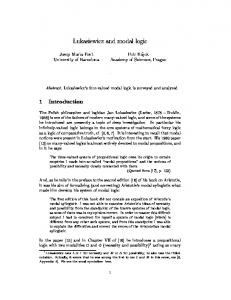
where φ : R → [0, 1] is a monotone-nondecreasing continuous function (referred to as activation function), ωok is the synaptic weight from neuron k in the l-th hidden layer to the single output neuron o, ωkj is the synaptic weight from neuron j in the (l − 1)-th hidden layer to neuron k in the l-th hidden layer, and so on for the other synaptic weights. A graphical representation of a multilayer perceptron is given by Figure 1.
f (x) =
u X
hfri(ri ) (x).
i=1
Lemma III.1: Let hsrii (with 1 < i < n) be a rational hat associated with the set {(r1 , s1 ), . . . , (rn , sn )}. Let ψ : R → [0, 1] be defined as ψ(x) = (1 ∧ x) ∨ 0. Then H : [0, 1] → [0, 1] defined as: ¶ µ ri −1 x+ H(x) = si ψ(1) − si ψ ri − ri−1 ri − ri−1
µ −
si ψ
1 ri x− ri+1 − ri ri+1 − ri
¶ ,
is such that hrsii = H. Proof: The hat hsrii has the form: 0 x − ri−1 si hsrii (x) = ri − ri−1 r −x si i+1 ri+1 − ri
for x ∈ [0, ri−1 ] ∪ [ri+1 , 1] for x ∈ [ri−1 , ri ] for x ∈ [ri , ri+1 ]
ri −1 Let ∆l (x) = ri −r x + ri −r , and ∆r (x) = ri+11−ri x − i−1 i−1 ri ri+1 −ri . Then H(x) = si − si ψ(∆l (x)) − si ψ(∆r (x)). Now there are four cases: • When x ∈ [0, ri−1 ], ∆l (x) ≥ 1 and ∆r (x) < 0. Then H(x) = 0. • When x ∈ [ri−1 , ri ], 0 ≤ ∆l (x) ≤ 1 and ∆r (x) < 0. Then i−1 i −x H(x) = si − si rir−r = si rx−r . i−1 i −ri−1 • When x ∈ [ri , ri+1 ], ∆l (x) < 0 and 0 ≤ ∆r (x) ≤ 1. Then i+1 −x H(x) = si rri+1 −ri . • When x ∈ [ri+1 , 1], ∆l (x) < 0 and ∆r (x) ≥ 1. Then H(x) = 0.
The above Lemma can be easily extended to Schauder hats hsr11 and hsrnn . In the following we shall refer to nets like H as (Schauder) hat nets, because they shall play for neural networks the same role that rational hats play in Rational L Ã ukasiewicz logic. Theorem III.2: Let ψ : R 7−→ [0, 1] be defined as ψ(x) = (1 ∧ x) ∨ 0. Then: (i) For all n ¯ ∈ N, αi , wij , bi ∈ Q, where i = 1, . . . , n ¯, F : [0, 1] 7−→ [0, 1] defined as: F (x) =
n ¯ X
αi ψ (wi x + bi )
1=1
is a rational McNaughton function. (ii) For any rational McNaughton function f , there exist n ¯ ∈ N and αi , wi , bi ∈ Q, where i = 1, . . . , n ¯ and j = 1, . . . , n, such that f (x1 , . . . , xn ) =
n ¯ X
αi ψ (wi x + bi ) .
1=1
Proof: (i). The function ψ is a piecewise linear function and ψ (wi xi + bi ) is a piecewise linear function. Since a sum of a finite number of Pn¯piecewise linear function is a piecewise linear function, 1=1 αi ψ (wi xi + bi ) is again a piecewise linear function taking values in [0, 1]. Hence it is a rational McNaughton function. (ii). Every rational McNaughton function f can be represented as a weighted sum of rational hats. Since from Lemma III.1 it is possible to associate to each hat h a hat net H, f can be represented by a weighted hat nets.
B. The n-dimensional case In order to extend Theorem III.2 to the n dimensional case, we need some preliminary results: Lemma III.3: The activation function ψ maps any finite weighted sum of rational McNaughton functions (where the weight are rational values) into a rational McNaughton function. Proof: Let f, f1 , f2 be rational McNaughton functions and p, p1 , p2 , q, q1 , q2 be natural numbers. Then it is easy to check that: ψ(f ) ψ(f1 + f2 ) ψ(f1 − f2 ) p ψ( f ) q p1 p2 ψ( f1 − f2 ) q1 q2
= = =
f f1 ⊕ f2 f1 ª f2
=
pδq f
=
p1 δq1 f1 ª p2 δq2 f2
We want now to associate a neural network to each Rational L Ã ukasiewicz formula of n variables. We could extend the concept of Schauder hats to the n-dimensional case, but as already mentioned, the description for such hats is very complicate. We shall give an alternative method based on the proof of McNaughton representation theorem as presented in [1]. Let f : [0, 1]n → [0, 1] be a piecewise linear function and let p1 , . . . , pu be the linear functions that are the pieces of f in the sense that for every x ∈ [0, 1]n there exists i ∈ {1, . . . , u} such that f (x) = pi (x). Let Σ denote the set of permutations of {1, . . . , u} and for every σ ∈ Σ let Pσ = {x ∈ [0, 1]n | pσ(1) (x) ≤ . . . ≤ pσ(u) (x)}. In other words Pσ is a polyhedron such that the restrictions of linear functions p1 , . . . , pu to Pσ are totally ordered, increasingly with respect to {σ(1), . . . , σ(u)}. We denote by iσ the index such that f (x) = pσ(iσ ) (x)
for every x ∈ Pσ .
The proof of the following theorem can be found in [1]. Theorem III.4: For every x ∈ [0, 1]n , f (x) = min max pσ(j) (x) = min max ψ(pσ(j) (x)). σ∈Σ 1≤j≤iσ
σ∈Σ 1≤j≤iσ
By using neural networks we can express linear combinations, but we need to define networks corresponding to minimum and maximum. Proposition III.5: For every x, y ∈ [0, 1], one-layer neural networks F1 (x, y) F2 (x, y)
= ψ(y) − ψ(y − x) = ψ(y) + ψ(x − y)
coincides respectively with min(x, y) and max(x, y). Proof: If x ≤ y then ψ(y) = y, ψ(y − x) = y − x and ψ(x − y) = 0, hence F1 (x, y) = x and F2 (x, y) = y.
If y ≤ x then ψ(y) = y, ψ(y−x) = 0 and ψ(x−y) = x−y, hence F1 (x, y) = y and F2 (x, y) = x. We can hence describe neural representation of McNaughton functions. Theorem III.6: (i) For every l, n, n(2) , . . . , n(l) ∈ N, and ωij , bi ∈ Q, the function F : [0, 1]n 7−→ [0, 1] defined as F (x1 , . . . , xn ) = (l−1) (l) n nX ³ X φ ωok φ ωkj φ . . . j=1
k=1
à n X
! ωli xi + bi
and GFED / @ABC ψ L LL A £ L £ 1 LL £ £ £ rr ££ −1 rr ££ rr 1 GFED / @ABC ψ Y X
1
/ Max(X,Y)
1
1. Consider the formula (x ⊕ y) ¯ (¬(x ⊕ y) ⊕ 2x), whose truth table is given by Figure 2.
!!! ...
,
i=1
is a rational McNaughton function. (ii) For any rational McNaughton function f , there exist l, n, n(2) , . . . , n(l) ∈ N, and ωij , bi ∈ Q such that f (x1 , . . . , xn ) = (l) (l−1) n nX ³ X φ ωok φ ωkj φ . . . j=1
k=1
à n X
! ωli xi + bi
1 0.75
1
0.5 0.25 0 0
0.75 0.5 0.25 0.25
0.5 0.75
!!! ...
10
.
i=1
Proof: (i) By Lemma III.3. (ii) By Theorem III.4 we have
Fig. 2. The rational McNaughton function associated to the formula (x ⊕ y) ¯ (¬(x ⊕ y) ⊕ 2x)
Such function is equal to (3x ∧ 1) ∧ ((x + y) ∧ 1) hence the corresponding neural network will be as in Figure 3.
f (x) = min max ψ(pσ(j) (x)). σ∈Σ 1≤j≤iσ
For every σ and j, the function ψ(pσ(j) (x)) is a network with one hidden layer. Then applying networks as in Proposition III.5 we get the claim. Corollary III.7: The class of neural networks as in Theorem III.6 is dense in the class of multi-layer perceptrons representing continuous functions. Proof: By using a simple variation of Weierstrass theorem [8] it is possible to show that rational McNaughton functions are able to approximate every continuous function with an error as low as desired. Then, by the previous theorem we get the claim. From the corollary it follows that the use of only truncated identity ψ as activation function is not a severe restriction on the the class of neural networks which can be obtained; they can approximate every neural network representing a continuous function.
−1
2
GFED @ABC / GFED / @ABC ψ K ψ X; KK−1 @ ;; ¡ KKK ;; 1 ¡¡ K% 2 ¡ ;; ¡ s9 ¡ s ;; ¡ s s À ¡¡ sss1 @ABC GFED GFED @ABC / / ψ ψ Y /
1
1
Fig. 3. The neural network representing the formula (x ⊕ y) ¯ (¬(x ⊕ y) ⊕ 2x)
2. The McNaughton function ((x ⊕ δ3 x) ∨ 2y) ∧ (2x ∨ 2¬y) whose graphic is given by Figure 4, corresponds to neural network in Figure 5.
C. Examples In this section we shall give some examples of the previous theorem. First of all note that networks corresponding to min(x, y) and max(x, y) are given by
1 0.75
1
0.5 0.25 0 1
0.75 0.5
0.75
@ABC ψ L X −1 / GFED LL £A L £ −1 LL £ £ £ rr ££ 1 rr r ££ r 1 GFED / @ABC ψ Y 1
0.5
0.25 0.25
/ Min(X,Y)
00
Fig. 4. Graphic of ((x ⊕ δ3 x) ∨ 2y) ∧ (2x ∨ 2¬y)
@ABC GFED GFED / @ABC ψ K : ψ 1 KKK B u J u ¹ ¦ K u 1 K% ¦¦ uu 1/3¹ ¦ @ABC GFED @ABC / GFED ¹ ¦ ψ ψ X. II ¹ −1 s9 ¦¦ −1 9 .. II ¹¹ s I ¦ s µ 999 ¦ ss1 ..1 I¹ $ s µ 99 µ @ABC GFED / @ABC .. ¹¹ GFED ψ ψ −1 99 1 µµ .¹.¹ ³G 9¿ µ 1 ¹ .1 ³ µµµ ¹¹ ..³ @ABC GFED ³. ψ µµµ 1 B ¹¹¹ ³³³ .º ¦ µ ¦¦ ¹ ³³ 1/3 @ABC GFED GFED / @ABC µµ ¦¦1 ψ K ¹¹¹ ³³ u: ψ µ ¦ 1 KKK ¦ B ³ u µµ K ¦¦ ¦¦ ¹³¹ ³uuu1/5 1 K% ¦ @ABC @ABC GFED / GFED ¦¦ ψ ψ Y II 1 s9 ¦¦ −1 II s ¦ s s I ¦ s s 1 −2 $ GFED @ABC GFED / @ABC ψ ψ 7 1 p p ppp2 1 Fig. 5. Neural network corresponding to function of Figure 4
IV. Conclusions The learning process is one of the most distinguished feature of NN. However there are some drawbacks. Learning has a cost. Thus when we deal with complex systems, we need to reduce this cost. We can use a NN to learn a model. But we have no tools to use what has been obtained for simplifying the learning of a slightly different model. For example we could think that the synaptic weights of the NN associated to this new model are for the most part the same of the old NN. However we have nothing to do, but to start from scratch. Each learning has an history per se, we cannot learn from learning. Moreover many times, beside a set of examples (like experimental data), other information (partial mathematical model, linguistic description) is available about the system we want to model. It should be very useful to use this kind of information to reduce the search space for the optimal network. Unfortunately actually there are no well defined methodologies suitable for incorporate a priori information in the network structure. At most there exist some ad hoc highly specific procedures In this paper we shown that it is possible to represent NN with a saturating linear transfer function and rational weights as formulas of a given logic (rational L Ã ukasiewicz logic) and viceversa. In this way we can integrate different kind of knowledge in the NN and divide a NN in subnetworks, each responsible of a certain behavior. Moreover, from the point of view of logic, now it is possible to associate to each formula an analog circuit. Thus, although we did not yet define a normal form, we made a step in this direction and gave the possibility to physically implement the formulas of rational L Ã ukasiewicz logic. References [1] S. Aguzzoli. Geometrical and Proof Theoretical Issues in L Ã ukasiewicz propositional logics. PhD thesis, University of Siena, Italy, 1998.
[2] J.L. Castro and E. Trillas. The logic of neural networks. Mathware and Soft Computing, 5:23–27, 1998. [3] B. Gerla. Functional representation of many-valued logics based on continuous t-norms. PhD thesis, University of Milano, Italy, 2000. [4] B. Gerla. Rational L Ã ukasiewicz logic and Divisible MV-algebras. Neural Networks World, 11:159, 2001. [5] S. Haykin. Neural Neworks – A Comprehensive Foundation. Prentice-Hall, London, 1999. [6] R. McNaughton. A theorem about infinite-valued sentential logic. The Journal of Symbolic Logic, 16(1):1–13, 1951. [7] D. Mundici. A constructive proof of McNaughton’s theorem in infinite-valued logics. Journal of Symbolic logic, 59:596–602, 1994. [8] P. Amato and M. Porto. An algorithm for the automatic generation of a logical formula representing a control law. Neural Nerwork World, 10(5):777–786, 2000.