New Top-Down Methods Using SVMs for Hierarchical

New Top-Down Methods Using SVMs for Hierarchical Multilabel Classification Problems Ricardo Cerri and André Carlos P. L. F de Carvalho

Abstract— Hierarchical Multilabel Classification is a problem where examples can be assigned to more than one class simultaneously and the classes are hierarchically structured. This paper describes and evaluates five different methods for this classification task, based on two approaches, named topdown and one-shot. In the top-down approach, the classification task is carried out by discriminating the classes, level by level, in the hierarchy. In the one-shot approach, the methods consider the whole set of classes at once in the classification. Based on the top-down approach, two new hierarchical methods (with label combination and with label decomposition) and the well known binary hierarchical method are investigated using SVM classifiers. Other two methods from the literature, named HC4.5 and Clus-HMC, based on the one-shot approach, are also used. The methods are applied to ten biological datasets and evaluated using specific metrics for this kind of classification. The experimental results show that the proposed methods can improve the classification accuracy.

I. I NTRODUCTION In traditional classification problems, each example is associated with just one of two or more classes. The task of hierarchical multilabel classification (HMC) is more complex, since the classes are structured in a hierarchy and examples can belong to more than one class simultaneously. These problems are very common, for example, in the classification of genes, identification of protein functions and text classification. Many methods have been proposed in the literature to deal with HMC problems. The majority of them are applied to protein and gene function prediction [1], [2], [3], [4], [5], [6], [7] and text classification [8], [9], [10]. The HMC problem can be treated using two approaches, named top-down or local, and one-shot or global. In the top-down approach, during the training phase, the hierarchy of classes is processed level by level, producing one or more classifiers for each level of the hierarchy. This process produces a tree of classifiers. The root classifier is induced with all training examples. In the next level, a classifier is induced using just the examples belonging to the classes predicted by the previous classifier in the hierarchy. In the test phase, when an example is assigned to a class that is not a leaf in the hierarchy, it is further classified into one or more subclasses of this class. A disadvantage of this Ricardo Cerri is with the Department of Computer Sciences, University of São Paulo, Campus São Carlos, Av. Trabalhador São-carlense, 400, Centro, P.O.Box: 668, CEP: 13560-970, São Carlos, SP, Brazil (phone: +55 16 33738161; email: [email protected]). André de Carvalho is with the Department of Computer Sciences, University of São Paulo, Campus São Carlos, Av. Trabalhador São-carlense, 400, Centro, P.O.Box: 668, CEP: 13560-970, São Carlos, SP, Brazil (phone: +55 16 3373-9691; email: [email protected]).

approach is the propagation of errors through the levels of the hierarchy. However, it has the positive aspect that any traditional classification algorithm can be used. The one-shot approach induces an unique classification model considering the class hierarchy as a whole. For this reason, it presents a higher complexity in its implementation, but avoids the error propagation problem, present in the topdown approach. After the induction phase of the algorithm, the prediction of classes for a new example occurs in just one step. Hence, traditional classification algorithms cannot be used, unless adaptations are made to consider the whole hierarchy of classes. This paper describes and evaluates five methods based on the top-down and one-shot approaches. The first method, named HMC-Binary-Relevance (HMC-BR), is well known from the literature, and is based on top-down binary classification. The second and third methods, proposed in this work, are new variations of non-hierarchical multilabel methods, and are named HMC-Label-Powerset (HMC-LP) - based on top-down combination of labels -, and HMC-Cross-Training (HMC-CT) - based on top-down label decomposition. The other two methods are named HC4.5 [1] - a hierarchical multilabel extension of the C4.5 algorithm [12] -, and ClusHMC [6] - based on the concept of Predictive Clustering Trees [15]. Support Vector Machines (SVMs) [20] were used in the top-down approach. The experiments were performed using ten datasets with gene functions of the Saccharomyces cerevisiae organism, describing different data conformations. The following sections are organized as follows: Section II formally presents the HMC problem; the HMC methods compared are explained in Section III; Section IV presents the materials and methods; the experiments are reported in Section V, with an analysis of the results obtained; finally, Section VI presents the main conclusions and future works. II. H IERARCHICAL M ULTILABEL C LASSIFICATION The HMC problem is formally defined as follows [11]: Given: a space of examples Y and a class hierarchy (C, ≤h ), where C is a set of classes and ≤h is a partial order representing the superclass relationship (for all c1 , c2 ∈ C : c1 ≤h c2 if and only if c1 is a superclass of c2 ); a set T of examples (yi , Si ) with yi ∈ Y and Si ⊆ C such that c ∈ Si ⇒ ∀c0 ≤h c : c0 ∈ Si ; a quality criterion q that rewards models with high accuracy and low complexity. Find: a function f : Y → 2C , where 2C is the powerset of C, such that c ∈ f (y) ⇒ ∀c0 ≤h c : c0 ∈ f (y) and f maximizes q.

An example of HMC problem is illustrated in Figure 1, where the class hierarchy is represented as a tree. A newspaper report can, for example, address subjects related to computer sciences and collective sports and thus be classified in both sciences/computing and sports/collective/soccer. The prediction of an example generates a subtree.

Fig. 1. HMC problem structured as a tree. (a) Class hierarchy. (b) Predictions generating a subtree.

The quality criterion q can be based on the distance between the classes in the hierarchy. It can be, for example, the mean precision of the different classes predicted, or it can consider that classification errors in levels of the hierarchy closer to the root are worse than errors in deeper levels [3]. The next section presents the methods used in this paper. III. H IERARCHICAL M ULTILABEL M ETHODS A. HC4.5 This method, proposed by [1], is a variation of the C4.5 algorithm [12], where the authors reformulated the entropy formula using the sum of the entropies of all classes. The entropy can be defined as the amount of necessary information to describe an example of the dataset. It is equivalent to the amount of necessary bits to describe all the classes that belong to an example. This new formulation of the entropy allows the leaves of the decision tree to be a set of labels. Thus, the classification output for a new example can be a set of classes represented as a vector. The induction of the model is done in just one step, and generates one decision tree for the whole hierarchy. This process of induction is more complicated. However, a simple set of rules is generated. The new entropy formula is presented in Equation (1) [13]:

entropy(S) = −

N X

((p(cj ) log2 p(cj )) + (q(cj ) log2 q(cj ))

j=1

− α(cj ) log2 treesize(cj ))

(1)

where • N = number of classes of the problem; • p(cj ) = probability (relative frequency) of class cj ; • q(cj ) = 1 - p(cj ) = probability of not being member of class cj ; • treesize(cj ) = 1 + number of descendant classes of class cj (1 is added to represent cj itself);

α(cj ) = 0, if p(cj ) = 0 (a user-defined constant (default = 1) otherwise). The final output of HC4.5, for a given example yi , is a vector of real values vi . If the value of vi,j is above a given threshold l, the example is assigned to the class cj . The original HC4.5 can automatically assign a new example to a class in any level of the hierarchy, depending on the characteristics of the data at each level. Since the goal of this paper is to do an experimental comparison of the one-shot and top-down approaches in a way which is as controlled as possible, the HC4.5 method used in the experiments was modified in the work [14]. This version of the algorithm includes the restriction that it always assigns a new example to a class in a leaf node of the class tree, which is the prediction process used in this work. The method is implemented in the C programming language. The program can be obtained upon authors’ request, due distribution restrictions in the original C4.5 code. •

B. Clus-HMC In this HMC method, decision trees are built using a framework named Predictive Clustering Trees (PCTs) [15]. In this framework, decision trees are constructed as a cluster hierarchy, in which the root node contains all the training examples, and is recursively partitioned in small clusters, as the decision tree is transversed toward the leaves. The PCTs can be applied both to the task of clustering and classification, and the procedure used to construct them is similar to other decision tree induction algorithms, like CART (Classification and Regression Trees) [16] or C4.5. Initially, the labels of the examples are represented as boolean vectors. Given an example, the j th position of its vector of classes receives the value 1 if the example belongs to the class cj , and 0 otherwise. The vector that contains the arithmetic mean, or prototype, of a set of vectors V , denoted by v, has, as its j th element, the proportion of examples of the set that belongs to the class cj . The variance of a set of examples Y , shown in Equation (2), is given by the mean square distance between each vector of classes vi of the examples and the vector of proportion of classes v. P d(vi , v)2 (2) V ar(Y ) = i |Y | To consider the depth of the classes in the hierarchy, i.e., classes at deeper levels represent more specific information than classes at higher levels, the weighted Euclidean distance between the classes was used. The calculation of this distance is shown in Equation (3), where vi,j is the j th element of the vector of classes vi of a given example yi , and the weights w(c) decrease as the depth of the classes in the depth(c) hierarchy increases (w(c) = w0 , with 0 < w0 < 1). The heuristic used to choose the best test t to be placed in a tree node is the maximization of the variance reduction of a set of examples [6]. sX d(v1 , v2 ) = w(cj ) × (v1,j − v2,j )2 (3) j

Different from a common decision tree, in a PCT, a leaf stores the mean v of the vector of classes of the examples of that leaf, i.e., the function that obtains the prototype of a group of examples returns the vector v. The proportion of examples in a leaf that belongs to a class cj is denoted by vj , and can be interpreted as the probability of an example be assigned to a class cj . When an example gets to a leaf of the decision tree, if the value of vj is above a given threshold lj , the example is assigned to the class cj . To ensure the integrity of the hierarchical structure, i.e., to ensure that when a class is predicted its superclasses are also predicted, the threshold values must be chosen in a way that lj ≤ lk always that cj ≤h ck , i.e., always that cj is a superclass of ck . The Java programming language was used in the implementation of Clus-HMC. The program used was implemented in the work [6], and is freely available at http: //www.cs.kuleuven.be/˜dtai/clus/. C. HMC-Binary-Relevance (HMC-BR) This method uses N classifiers in the induction phase, where N is the number of classes in the hierarchy. Each classifier is associated with one class and trained to solve a binary classification problem, using an one-against-all strategy. When a classifier is trained, the class associated with it is considered positive, and all the other classes are considered negatives. The method was originally proposed for non-hierarchical multilabel classification problems. In a HMC problem with four levels, with 2/3/4/5 classes on each level, two classifiers are trained in the first level, three in the second, four in the third, and five in the fourth level. In the first level, the problem is transformed into two binary classification problems, one for each class. The j th classifier considers the examples belonging to the j th class as positives and the other examples as negatives. Each classifier becomes specialized in the classification of a particular class. When a new example is presented, the classes for which the classifiers present a positive output are assigned to it. The same process is done in the other levels of the hierarchy. From the second level onwards, when a classifier is trained for a class cj , the training process is carried out considering only the examples that belong to the parent class of the class cj . This process is repeated until a leaf is reached. In the end of the process, a hierarchy of classifiers is obtained, and the classification of a new example occurs in a topdown manner. In the first class of the first level, when an example is assigned to a class cj , the algorithm is recursively called to submit the example to other classifiers that predict which subclasses of the class cj the example belongs to. This process is repeated for all classes of the hierarchy. The disadvantage of this method is that it assumes that the classes are independent from each other. This is not always true, and by ignoring possible correlations between classes, a poor generalization ability may be obtained. Additionally, the number of rules generated is high and the rules become more complex, since a decision tree is generated for every class in the hierarchy. The induction time is also high, due

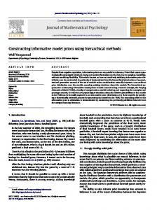
the large number of classes involved in the problem. On the other hand, the classification process is done in a natural and easier manner, as discriminating classes level by level is a classification method closer of what a human being would do, dealing with less classes at the same time. D. HMC-Label-Powerset (HMC-LP) This new method uses a combination of classes in order to transform the hierarchical multilabel problem in a hierarchical single-label problem. It considers the correlations between the classes in order to overcome the disadvantage of the HMC-BR method. The HMC-LP method is a hierarchical adaptation of a nonhierarchical multilabel classification method named LabelPowerset, used in the works [17] and [18]. For each example, the method combines all the classes assigned to it, at a specific level, into a new and unique class. Given an example belonging to classes A.D and A.E, and other example belonging to classes B.F , B.G, C.H and C.I, where A.D, A.E, B.F , B.G, C.H and C.I are hierarchical structures such that A ≤h D, A ≤h E, B ≤h F , B ≤h G, C ≤h H and C ≤h I with A, B and C belonging to the first level and D, E, F , G, H and I belonging to the second level, the resulting combination of classes for the two examples would be a new hierarchical structure CA .CDE and CBC .CF GHI , respectively. In the example, CDE is a new label formed by the combination of the labels D and E, and CF GHI is a label formed by the combination of the labels F , G, H and I. Figure 2 illustrates this process of label combination. To the best of our knowledge, such adaptation was not yet reported in the literature.

Fig. 2.

Label combination process of the HMC-LP method.

After the combination of classes, the original HMC problem is transformed into a hierarchical single-label problem, and a top-down approach is employed, using one or more multiclass classifiers per level. In the end of the classification, the original multilabel classes are recovered. The correlation between classes is considered in this method, but the combination of labels can considerably increases the number of classes, and some of them may end up with few examples. The induction time, however, decreases compared with the HMC-BR method, as fewer classifiers have to be trained. The label combination procedure is presented in the Algorithm 1. E. HMC-Cross-Training (HMC-CT) This method, also proposed in this work, uses a label decomposition process, where all multilabel examples are decomposed into a set of single-label examples. In this process, for each example, each possible class is considered

Algorithm 1: Label combination procedure of HMC-LP. Procedure LabelCombination(Y, C) Input: set of examples Y , set of classes C Output: N ewClasses 1 foreach level j of the class hierarchy do 2 foreach subset Ci of the set C, assigned to an example yi in level j do 3 Gets a new class ci,j for the example yi from Ci 4 N ewClassesi,j ← ci,j 5

return N ewClasses

as the positive class in sequence, using the multilabel data more than once during the training phase. As an example, if a dataset has multilabel examples with labels A, B and C, when a classifier for class A is trained, all the multilabel examples whose set of classes includes A become singlelabel examples for class A. The same happens to the other classes. The method was originally proposed by [19] for nonhierarchical multilabel problems and named Cross-Training. For this new hierarchical variation of Cross-Training, the process of label decomposition is applied to all levels of the hierarchy, and a top-down strategy is followed during the training and test phases. Figure 3 shows an example of the label decomposition process applied by the HMC-CT method in a dataset. When an example belongs to more than one class, these classes are separated by a slash (/).

Fig. 3.

Label decomposition process of the HMC-CT method.

It is important to notice that HMC-CT is different from HMC-BR. In HMC-CT, a classifier is not associated with each class, transforming the original problem into a binary problem. Instead, multiclass classifiers are used, because all classes participate in the training process. The difference is that, for an example yi , if this example belongs to two classes, A and B, the training process occurs twice, once considering the example as belonging to class A and another time considering the example as belonging to class B. Algorithm 2 shows the classification process of HMC-CT. A problem with this method is the induction time, which

Algorithm 2: Classification process of HMC-CT. Procedure Classify(y, Cl) Input: example y, set of classifiers Cl Output: Classes 1 Classes ← ∅ 2 foreach classifier cli from the set of classifiers Cl do 3 Predicts a class ci for the example y using the classifier cli 4 if not the last hierarchical level then 5 Gets the set Cli of children classifiers of the classifier cli trained with examples from class ci 6 Classes ← Classes ∪ {ci }∪Classify(y, Cli ) 7 else 8 Classes ← Classes ∪ ci 9

return Classes

greatly increases compared with the other methods. This is because the training process occurs several times, using the same examples several times, considering all classes that belong to the examples. IV. M ATERIALS AND M ETHODS A. Support Vector Machines The SVMs [20] are based on the statistical learning theory, and use non-linear kernel functions to map the vectors of characteristics of the examples to a space of higher dimension, usually much larger than the original space [21]. With an appropriate mapping for a large enough dimension, it is possible to separate data from two classes by a hyperplane. In classification problems with more than two classes, two strategies are used. The first one is known as one-against-all, where the problem is decomposed in N binary problems, being N the number of classes. A binary classifier is then associated with each class and specialized in separate its associated class from all other classes. The second strategy is named one-against-one, and uses N (N −1)/2 binary classifiers, where each classifier is used to distinguish between a pair of classes. The objective of the training of the SVMs is to find a hyperplane to separate data from different classes with the largest possible margin. It is expected that the greater the margin, the greater the generalization ability of the classifier. The margin of separation between classes is a fundamental concept in the design of SVMs and is associated with the allowable error in the classification. The examples that are within the margin of separation or on it are called support vectors and define the dividing surface. Figure 4 ilustrates an example of a separating hyperplane. The choice of SVMs as the classifiers used in the top-down methods of this work was motivated by their good generalization ability, even for problems with many attributes. B. Datasets The datasets used in the experiments reported in this paper are related to gene functions of the Saccharomyces

Fig. 4.

Example of a Separating Hyperplane of SVMs.

cerevisiae fungus, often used in the fermentation of sugar for the production of ethanol, and also in the fermentation of wheat and barley for the production of alcoholic beverages. It is one of the biology’s classic model organisms, and has been subject of intensive study for years [6]. The datasets are structured as a tree according to the FunCat (http://mips.gsf.de/projects/ funcat) scheme developed by MIPS [22], and are freely available at http://www.cs.kuleuven.be/ ˜dtai/clus/hmcdatasets.html. The Funcat annotation scheme consists of 28 main categories that cover fields such as cellular transport, metabolism and cellular communication. Its hierarchy is structured as a tree, with up to six levels deep and a total of 1632 functional classes. Table I shows the main characteristics of the datasets used. Due the high computational cost of the experiments when using the original datasets, a sample of each dataset was used. The experiments were performed using four subtrees of each dataset. The four subtrees are rooted in the classes 01, 02, 10 and 11, respectively. These subtrees were randomly selected. Additionally, four of the six levels of the original datasets were considered.

N. Examples. Tot. Mult. 2444 1451 2445 1451 2441 1449 2438 1449 1579 988 2444 1450 2454 1456 1059 634 2480 1477 2419 1439

Avg. N. Ex. L1 L2 611.0 111.1 611.2 111.1 610.2 110.9 609.5 110.8 394.7 71.7 611.0 111.0 613.5 111.5 264.7 48.1 620.0 112.7 604.7 109.9

per Class L3 L4 29.7 17.4 29.7 17.4 29.7 17.4 29.6 17.3 21.3 13.1 29.7 17.4 29.8 17.4 13.6 8.1 30.2 17.6 29.4 17.2

Class N. L1 L2 1.3 1.6 1.3 1.6 1.3 1.6 1.3 1.6 1.3 1.7 1.3 1.6 1.3 1.6 1.4 1.7 1.3 1.6 1.3 1.6

X

Con(yi , cj ) =

(1.0 −

c0 ∈yi .lbc •

Avg. per Ex. L3 L4 1.4 0.9 1.4 0.9 1.4 0.9 1.4 0.9 1.5 1.0 1.4 0.9 1.4 0.9 1.4 0.9 1.4 0.9 1.4 0.9

Dis(c0 , cj ) ) Disθ

(4)

Dis(c0 , cj ) ) Disθ

(5)

If yi is a false negative: X

Con(yi , cj ) =

(1.0 −

c0 ∈yi .agc

TABLE I C HARACTERISTICS OF THE DATASETS

N. Atrib. Expr 551 CellCycle 77 Church 27 Derisi 63 Eisen 79 Gasch1 173 Gasch2 52 Phenotype 69 Sequence 478 SPO 80

The metrics used are based on the distances between the predicted and the real classes in the hierarchy tree, which are defined by the number of links between them. These metrics were proposed by [23] and are called Hierarchical Weighted Micro Average Precision and Recall. They take into account that classes closer in the hierarchy tend to be more similar to each other than classes more distant, and that predictions in deeper levels are more difficult. To represent this difficulty, weights are used in the links between the classes in the hierarchy. The weights used were (0.26, 0.13, 0.07, 0.04), where 0.26 is the weight of a link between the root node and any class of the first level, 0.13 is the weight of a link between a class in the first level and any of its subclasses, and so on. These weights were used originally in [24]. The metrics compute the contribution of a misclassified example to a given class using an acceptable distance Disθ , which must be specified and be greater than 0. If Disθ = 1, the misclassification of an example, whose predicted and real classes are connected by more than 1 link, will result in negative contribution, and zero contribution at 1 link. In the experiments, Disθ = 2 was used, so the misclassification of an example whose predicted and real classes are connected by 2 links results in zero contribution, and in negative contribution at more than two links. As it is not sufficient to evaluate the classification methods using only precision or recall, the F1 metric, that combines both metrics, was used. The contribution of an example yi to a class cj based on class distance is formally defined in Equations (4) and (5), where yi .agc and yi .lbc are respectively the predicted and real classes of example yi . • If yi is a false positive:

The contribution of an example yi is then refined to be restricted to the range of [−1, 1]. This refinement, denoted by RCon(yi , cj ), is defined in Equation (6). RCon(yi , cj ) = min(1, max(−1, Con(yi , cj )))

(6)

For all the examples, the total contribution of false positives (F pConj ) and false negatives (F nConj ) are defined in Equations (7) and (8). X F pConj = RCon(yi , cj ) (7) yi ∈F Pj

C. Evaluation of the Classification Methods The evaluation was carried out level by level in the classification hierarchy. For each hierarchical level, a value resulting from the evaluation of the predictive performance in the level was reported.

F nConj =

X

RCon(yi , cj )

(8)

yi ∈F Nj

Given the examples’ contributions, the Micro-Average Precision and Recall are defined in Equations (9) and (10).

PN

j=1 (max(0, |T Pj | + F pConj + F nConj )) PN j=1 (|T Pj | + |F Pj | + F nConj )

µDB Pˆr =

(9)

ˆ µDB = Re

PN

i=j (max(0, |T Pj | + F pConj + F nConj )) PN j=1 (|T Pj | + |F Nj | + F pConj )

(10) Since both F pConj and F nConj can be negative, |T Pj |+ F pConj + F nConj can be negative. Therefore, a max function is applied to the numerator to make it not less than 0. As F pConj ≤ |F Pj |, when |T Pj | + |F Pj | + F nConj ≤ 0, the numerator max(0, |T Pj | + F pConj + F nConj ) = 0, µDB and Pˆr can beµDB treated as 0 in this case. The same rule ˆ is applicable to Re [23]. µDB ˆ ˆ µDB , the hierarchical With the values of P r and Re F1 metric can be computed as shown in Equation (11). In the equation, β refers to the importance assigned to the values of µDB ˆ µDB . When the value of β is increased, the Pˆr and Re ˆ µDB is increased. When weight assigned to the value of Re the value of β is decreased, the weight assigned to the value µDB of Pˆr is increased. In this work, β = 1 was used, so µDB ˆ ˆ µDB have equal weights. Pr and Re µDB ˆ µDB (β 2 + 1) × Pˆr × Re F1 = µDB ˆ µDB β 2 × Pˆr + Re

(11)

For the evaluation, the real and predicted sets of classes of the examples are represented as boolean vectors, where each position of the vectors represents a class in the dataset. If an example belongs to a class cj , the j th position of the vector that represents the real set of classes receives the value 1. The same happens in the vector that represents the predicted set of classes. The datasets were divided using the 5-fold cross-validation technique, and statistical tests were applied to verify the statistical significance of the results, with significance levels of 90% and 95%. The tests employed were Friedman [25] and Nemenyi [26]1 , which are more adequate for comparisons involving many datasets and many classifiers [27].

dataset, are shown in bold face and the standard deviations are shown between parentheses. As can be seen in the table, the performances of the methods decrease as the level of the hierarchies become deeper. This is expected, because the prediction of classes is more difficult as the levels of the hierarchies become deeper, and the information obtained is more specific. Additionally, the problem of error propagation of the top-down approach contributes for its worse results in the last levels. TABLE II C OMPARISON OF TOP - DOWN AND ONE - SHOT APPROACHES Dataset

HMC-BR

CellCycle Church Derisi Eisen Gasch1 Gasch2 Phenotype Sequence SPO

49.6 57.4 44.3 47.5 58.1 59.9 55.3 46.0 45.3 50.1

(2.2) (2.1) (1.8) (1.4) (2.4) (2.1) (1.4) (3.0) (2.7) (1.6)

Expr CellCycle Church Derisi Eisen Gasch1 Gasch2 Phenotype Sequence SPO

30.9 33.1 23.5 24.9 34.3 38.0 30.5 26.3 29.7 26.8

(1.2) (2.0) (1.2) (0.5) (2.3) (2.4) (1.2) (2.3) (3.2) (1.1)


23.7 24.4 16.8 18.0 26.1 29.9 22.1 19.5 24.0 19.2

(1.4) (1.8) (1.0) (0.5) (1.8) (2.1) (0.4) (1.8) (3.0) (0.6)


20.3 21.5 14.2 15.2 23.0 26.1 19.3 16.8 21.8 16.7

(0.9) (1.4) (0.6) (0.6) (1.7) (1.8) (0.6) (1.9) (2.4) (0.8)

Top-down HMC-LP HMC-CT First Level 51.3 (1.7) 56.5 (1.0) 58.5 (2.7) 61.8 (1.6) 45.5 (1.2) 55.8 (1.6) 46.7 (1.5) 54.7 (1.9) 59.8 (1.2) 62.0 (2.9) 60.6 (1.7) 63.4 (2.1) 55.8 (1.0) 57.6 (0.7) 45.7 (1.9) 54.2 (1.6) 52.7 (2.4) 59.0 (0.9) 49.7 (1.9) 54.6 (1.5) Second Level 32.3 (2.0) 30.3 (1.3) 34.6 (3.4) 32.6 (2.0) 24.1 (0.9) 26.8 (1.8) 24.9 (1.2) 25.7 (1.3) 36.8 (1.4) 33.1 (3.5) 38.8 (2.1) 34.9 (2.6) 32.1 (0.9) 28.3 (0.5) 27.3 (1.4) 27.3 (1.7) 33.7 (1.9) 32.7 (0.7) 26.7 (1.8) 26.2 (1.8) Third Level 23.9 (1.4) 20.3 (1.2) 25.2 (2.8) 18.8 (1.3) 17.3 (0.5) 15.1 (0.8) 18.2 (0.7) 14.5 (0.6) 27.4 (1.7) 18.9 (1.8) 29.5 (1.9) 21.0 (1.7) 23.1 (0.8) 16.2 (0.4) 19.9 (0.5) 15.1 (1.3) 26.0 (1.3) 22.4 (0.7) 19.4 (0.7) 14.8 (0.7) Fourth Level 19.8 (1.3) 16.2 (0.8) 22.3 (2.5) 14.3 (1.1) 14.6 (0.4) 10.9 (0.7) 15.6 (0.8) 10.2 (0.4) 24.3 (1.5) 14.0 (1.4) 26.7 (1.8) 16.1 (1.6) 20.5 (1.0) 11.8 (0.4) 17.5 (0.7) 10.5 (0.8) 21.8 (1.1) 17.8 (0.7) 16.8 (0.8) 10.6 (0.4)

One-shot HC4.5 Clus-HMC 50.0 47.5 47.6 45.5 48.8 48.9 46.8 48.9 48.3 45.2

(1.5) (1.7) (1.2) (1.0) (1.7) (1.9) (1.6) (0.9) (1.7) (1.0)

51.7 47.1 47.3 46.2 50.6 49.5 47.4 47.4 49.1 45.8

(1.6) (1.6) (1.2) (2.3) (1.5) (1.6) (1.3) (1.7) (2.7) (1.9)

26.6 25.5 17.1 24.5 26.5 25.7 25.1 17.7 26.3 24.4

(0.7) (0.7) (1.1) (0.3) (1.0) (0.7) (0.8) (0.9) (0.8) (0.4)

27.9 26.1 18.9 25.4 27.7 27.1 26.0 19.8 27.2 25.6

(0.8) (0.6) (1.4) (0.9) (0.4) (0.9) (0.3) (2.0) (1.0) (0.7)

18.2 17.2 07.3 16.8 18.2 17.0 17.0 07.9 18.0 16.6

(0.6) (0.6) (0.5) (0.3) (1.0) (0.5) (0.6) (0.5) (0.5) (0.3)

19.6 18.4 09.2 18.2 19.6 19.2 18.4 12.1 20.2 18.1

(0.3) (0.2) (1.3) (0.5) (0.6) (1.0) (0.3) (2.7) (0.8) (0.3)

14.9 13.5 05.0 13.2 14.3 13.4 13.5 05.4 14.5 12.9

(0.9) (0.5) (0.3) (0.3) (0.9) (0.7) (0.6) (0.6) (0.4) (0.5)

16.7 15.1 06.4 15.0 16.7 15.9 15.3 09.0 17.9 14.7

(1.1) (0.4) (1.0) (0.7) (0.9) (1.2) (0.8) (2.6) (1.3) (0.2)

V. E XPERIMENTS AND D ISCUSSION For the experiments performed, the five hierarchical methods were compared. The R tool [28] was used in the implementation of the top-down methods, and the package e1071 [29] was used to generate the SVMs. The SVMs were used with a Gaussian kernel with the parameter values c = 100 and γ = 0.01. These values were suggested in previous works found in the literature, presenting good results. Table II shows the results obtained in the ten datasets in the four levels of the hierarchies. The best results, for each 1 The statistical tests used were implemented by Thiago Cov˜ oes, from the Bioinspired Computation Laboratory of ICMC/USP, São Carlos, SP, Brazil

The HMC-CT method achieved the best results in all datasets in the first level of the hierarchies. This may have occurred due the characteristics of the hierarchies in the first level. With just four classes in the first level, a high average number of examples per class and a low average number of classes per example, the classification process become easier. Additionally, by using the data more than once during the training phase, the datasets become less sparse, as neither a combination of labels nor a binary classification is applied in the method. According to the statistical tests, the differences between the HMC-CT method and the other methods was statistically significant.

In the other levels of the hierarchies, mainly in the third and fourth levels, the HMC-CT method achieved the worst results, together with HC4.5 and Clus-HMC methods. In the case of the HMC-CT method, as the number of classes in the second, third and fourth levels is higher than in the first level, and the training data is used many times, the number of predicted classes for each example becomes high, increasing the number of false positive examples. In the HC4.5 and Clus-HMC methods, the number of predicted classes for each example is also high, because no thresholds were used in the classification process. Due this fact, the number of errors committed for these two methods was high, i.e., the number of false positive examples increased. The higher is the number of false positives, higher is the classification recall and lower is the classification precision, harming the tradeoff between precision and recall, decreasing the value of the hierarchical F1 measure. The choice of not using threshold values is due the fact that, when the HC4.5 and Clus-HMC methods assign a value to a specific position vj of the vector of classes v of a given example, this assignment means that the classifiers assign to the example the corresponding class cj . The assigned value indicates only the probability of the pertinence of the class, and do not exclude it. In [6], Precision-Recall curves were used in the evaluation process of the classifiers based on PCTs, using many threshold values, so that the classifiers were compared based on the areas between the curves. This kind of evaluation was not used in this work because the other three methods do not assign real values do the vector of classes of an example, but only boolean values (0 and 1). In the second level of the hierarchies, the best results were obtained by the HMC-LP method. As the level of the hierarchies become deeper, the number of classes become higher, which makes the classification task more difficult for the HMC-BR method, that has to do a separate binary classification task for each class. In this case, the label combination process of the HMC-LP method can lead to better results, as can be seen in the majority of the datasets. Despite the different results of the methods HMC-BR, HMC-LP and HMC-CT, there were no statistically significant differences between them. Statistical differences were detected in the comparison with the methods HC4.5 and Clus-HMC. In the third and fourth levels of the hierarchies, the HMCLP also obtained the best results in almost all datasets, with exception of Gasch1 dataset in the third level, and Expr dataset in the fourht level. In these datasets, however, the performances of the methods HMC-LP and HMC-BR was practically the same. Again, due the high number of classes in the last levels, the label combination process seemed to favor the classification process of the HMC-LP method, producing a less sparse dataset for the training phase of the classifiers. It is also possible to see that, in the last levels of the hierarchies of some datasets, the methods HC4.5 and ClusHMC obtained some F1 values not so lower than the values obtained by the other three methods, and, in some cases, the results obtained by these two methods were higher than the

results obtained by HMC-CT. This may be due the problem of error propagation of the top-down approach, which is not present in the methods based on the one-shot approach. The results of the statistical tests showed that there were no statistically significant differences between the results of the HMC-BR and HMC-LP methods in the third and fourth levels of the hierarchies. Statistically significant differences were detected in the majority of the comparisons between the results of these two methods, and the results of the methods HMC-CT, HC4.5 and Clus-HMC. Table IV shows the results of the statistical tests applied in the experimental results. The symbols used for the interpretation of the tables are presented in Table III. These symbols represent the relationship between the results of the algorithms located in the rows of the tables with the algorithms located in the columns of the tables. TABLE III S YMBOLS USED IN THE RESULTS OF STATISTICAL TESTS Symbol N

M

Meaning Indicates that the performance of the algorithm located in the column was statistically better than the performance of the algorithm located in the row, with a significance level of 5%. Indicates that the performance of the algorithm located in the column was statistically better than the performance of the algorithm located in the row, with a significance level of 10%.

TABLE IV S TATISTICAL TESTS

HMC-BR HMC-BR HMC-LP HMC-CT HC4.5 Clus-HMC

N


N


HC4.5

Clus-HMC

Second Level HMC-LP HMC-CT

HC4.5

Clus-HMC

N N N Third Level HMC-LP HMC-CT

HC4.5

Clus-HMC

N N N Fourth Level HMC-LP HMC-CT

HC4.5

Clus-HMC

N N HMC-BR

HMC-BR HMC-LP HMC-CT HC4.5 Clus-HMC

First Level HMC-LP HMC-CT N M

N N

N N N

VI. C ONCLUSIONS In this paper, five methods for the hierarchical multilabel classification of bioinformatics data were compared. Two methods are based on the one-shot approach, which considers the whole set of classes at once when inducing a

classifier. Other three methods are based on the top-down approach, which discriminates the classes level by level in the hierarchy during the induction phase. In the top-down approach, the SVM machine learning algorithm was used. Two of the three top-down methods were proposed in this work, based on label combination and label decomposition, and are hierarchical variations of non-hierarchical multilabel methods of the literature. According to the experimental results, the variations in the standard top-down approach produced some of the best results, depending on the level being considered in the hierarchies and their multilabel characteristics. The HMCLP method was not only faster than HMC-BR and HMC-CT, but also achieved the best results in almost all hierarchical levels, showing to be a good alternative for HMC problems. In future works, other hierarchy structures, like Directed Acyclic Graphs (DAGs), can also be used. For this purpose, the classification methods need to be modified. A mechanism of correction of the error propagation problem of the top-down approach can also be implemented, which would certainly improve the performance of methods based on this approach. The use of threshold values can also be considered in the evaluation process. With the use of many threshold values, better performances could be obtained by the HC4.5 and Clus-HMC methods, because the values of the precision and recall metrics would vary, and a better tradeoff between them could be adjusted, increasing the value of the F1 metric. With this aim, classification algorithms that output real values could be used in the HMC-CT method. Finally, an analysis of how different classification methods are influenced by different hierarchical and multilabel characteristics of the datasets can also be done. Such study can help in the improvement of existing methods and in the development of new ones. ACKNOWLEDGMENT The authors would like to thank the Brazilian research councils FAPESP and CNPq for their financial support, the Katholieke Universiteit of Leuven’s Machine Learning Research Group for the datasets used and Thiago Covões for the codes of the statistical tests. R EFERENCES [1] A. Clare and R. D. King, “Predicting gene function in saccharomyces cerevisiae,” Bioinformatics, vol. 19, pp. 42–49, 2003. [2] H. Blockeel, M. Bruynooghe, S. Dzeroski, J. Ramon, and J. Struyf, “Hierarchical multi-classification,” in KDD-2002 Workshop Notes: MRDM, 2002, pp. 21–35. [3] J. Struyf, H. Blockeel, and A. Clare, “Hierarchical multi-classification with predictive clustering trees in functional genomics,” in Workshop on Computational Methods in Bioinformatics at the 12th Portuguese Conference on Artificial Intelligence, ser. LNAI, vol. 3808. Springer Berlin / Heidelberg, 2005, pp. 272–283. [4] Z. Barutcuoglu, R. E. Schapire, and O. G. Troyanskaya, “Hierarchical multi-label prediction of gene function,” Bioinformatics, vol. 22, no. 7, pp. 830–836, 2006. [5] R. Alves, M. Delgado, and A. Freitas, “Multi-label hierarchical classification of protein functions with artificial immune systems,” in III Brazilian Symposium on Bioinformatics, ser. LNBI, vol. 5167. Berlin, Heidelberg: Springer-Verlag, 2008, pp. 1–12.

[6] C. Vens, J. Struyf, L. Schietgat, S. Dˇzeroski, and H. Blockeel, “Decision trees for hierarchical multi-label classification,” Machine Learning, vol. 73, no. 2, pp. 185–214, 2008. [7] G. Valentini, “True path rule hierarchical ensembles,” in MCS ’09: Proceedings of the 8th International Workshop on Multiple Classifier Systems, ser. LNBI, vol. 5519. Berlin, Heidelberg: Springer-Verlag, 2009, pp. 232–241. [8] S. Kiritchenko, S. Matwin, and A. F. Famili, “Hierarchical text categorization as a tool of associating genes with gene ontology codes,” in Proceedings of the Second European Workshop on Data Mining and Text Mining in Bioinformatics, Pisa, Italy, 2004, pp. 30–34. [9] J. Rousu, C. Saunders, S. Szedmak, and J. Shawe-Taylor, “Kernelbased learning of hierarchical multilabel classification models,” J. Mach. Learn. Res., vol. 7, pp. 1601–1626, 2006. [10] N. Cesa-Bianchi, C. Gentile, and L. Zaniboni, “Incremental algorithms for hierarchical classification,” Machine Learning, vol. 7, pp. 31–54, 2006. [11] H. Blockeel, L. Schietgat, J. Struyf, S. Dzeroski, and A. Clare, “Decision trees for hierarchical multilabel classification: A case study in functional genomics.” in PKDD, ser. LNCS, J. Fürnkranz, T. Scheffer, and M. Spiliopoulou, Eds., vol. 4213. Springer, 2006, pp. 18–29. [12] J. R. Quinlan, C4.5: programs for machine learning. San Francisco, CA, USA: Morgan Kaufmann Publishers Inc., 1993. [13] A. Clare, “Machine learning and data mining for yeast functional genomics,” Ph.D. dissertation, University of Wales, 2003. [14] E. P. Costa, A. C. Lorena, A. C. Carvalho, A. A. Freitas, and N. Holden, “Comparing several approaches for hierarchical classification of proteins with decision trees,” in II Brazilian Symposium on Bioinformatics, ser. LNBI, vol. 4643. Berlin, Heidelberg: SpringerVerlag, 2007, pp. 126–137. [15] H. Blockeel, L. De Raedt, and J. Ramon, “Top-down induction of clustering trees,” in Proceedings of the 15th International Conference on Machine Learning. Morgan Kaufmann, 1998, pp. 55–63. [16] L. Breiman, J. Friedman, R. Olshen, and C. Stone, Classification and Regression Trees. Monterey, CA: Wadsworth and Brooks, 1984. [17] G. Tsoumakas and I. Vlahavas, “Random k-labelsets: An ensemble method for multilabel classification,” in Proceedings of the 18th European Conference on Machine Learning (ECML 2007), Warsaw, Poland, 2007, pp. 406–417. [18] M. R. Boutell, J. Luo, X. Shen, and C. M. Brown, “Learning multilabel scene classification,” Pattern Recognition, vol. 37, no. 9, pp. 1757–1771, 2004. [19] X. Shen, M. Boutell, J. Luo, and C. Brown, “Multi-label machine learning and its application to semantic scene classification,” in International Symposium on Electronic Imaging, San Jose, CA, 2004. [20] V. N. Vapnik, The Nature of Statistical Learning Theory (Information Science and Statistics). Springer-Verlag New York, Inc., 1999. [21] N. Cristianini and J. Shawe-Taylor, An Introduction to Support Vector Machines and Other Kernel-based Learning Methods. Cambridge University Press, 2000. [22] H. W. Mewes, D. Frishman, U. Güldener, G. Mannhaupt, K. Mayer, M. Mokrejs, B. Morgenstern, M. Münsterkötter, S. Rudd, and B. Weil, “Mips: a database for genomes and protein sequences.” Nucleic Acids Res, vol. 30, no. 1, pp. 31–34, 2002. [23] A. Sun and E.-P. Lim, “Hierarchical text classification and evaluation,” in Fourth IEEE International Conference on Data Mining, 2001, pp. 521–528. [24] N. Holden and A. Freitas, “Hierarchical classification of g-proteincoupled receptors with a pso/aco algorithm,” in Proc. IEEE Swarm Intelligence Symposium (SIS-06). IEEE Press, 2006, pp. 77–84. [25] M. Friedman, “The use of ranks to avoid the assumption of normality implicit in the analysis of variance,” Journal of the American Statistical Association, vol. 32, no. 200, pp. 675–701, 1937. [26] P. B. Nemenyi, “Distribution-free multiple comparisons,” Ph.D. dissertation, Princeton University, 1963. [27] J. Demˇsar, “Statistical comparisons of classifiers over multiple data sets,” Journal of Machine Learning Research, vol. 7, pp. 1–30, 2006. [28] R Development Core Team, R: A Language and Environment for Statistical Computing, R Foundation for Statistical Computing, Vienna, Austria, 2008. [Online]. Available: http://www.R-project.org [29] E. Dimitriadou, K. Hornik, F. Leisch, D. Meyer, and A. Weingessel, “r-cran-e1071,” 2008. [Online]. Available: http://mloss.org/software/ view/94/

New Top-Down Methods Using SVMs for Hierarchical

New Top-Down Methods Using SVMs for Hierarchical

Suggest Documents