network statistics in non-parametric Bayesian network models,. Bayesian non-parametrics does not address the third issue. (inferential complextiy) which is an ...
1
Non-parametric Bayesian modeling of complex networks
arXiv:1312.5889v1 [stat.ML] 20 Dec 2013
Mikkel N. Schmidt and Morten Mørup
Abstract—Modeling structure in complex networks using Bayesian non-parametrics makes it possible to specify flexible model structures and infer the adequate model complexity from the observed data. This paper provides a gentle introduction to non-parametric Bayesian modeling of complex networks: Using an infinite mixture model as running example we go through the steps of deriving the model as an infinite limit of a finite parametric model, inferring the model parameters by Markov chain Monte Carlo, and checking the model’s fit and predictive performance. We explain how advanced non-parametric models for complex networks can be derived and point out relevant literature.
I. I NTRODUCTION We are surrounded by complex networks. From the networks of cell interaction in our immune system to the complex network of neurons communicating in our brain, our cells signal to each other to coordinate the functions of our body. We live in cities with complex power and water systems and these cities are linked by advanced transportation systems. We interact within social circles and our computers are connected through the Internet forming the World Wide Web. To understand the structure of these large systems of biological, physical, social, and virtual networks, there is a great need to be able to model them mathematically [6]. Complex networks are studied in several different fields from computer science and engineering to physics, biology, sociology, and psychology. “Network science is an emerging, highly interdisciplinary research area that aims to develop theoretical and practical approaches and techniques to increase our understanding of natural and manmade networks” [6]. Network science can be considered “the study of network representations of physical, biological, and social phenomena leading to predictive models of these phenomena” [8]. To understand the many large-scale complex networks we sample and store today, there is a growing demand for advanced mathematical and statistical models that can account for the structure in these systems. The modeling aims are twofold; to provide a comprehensible description (i.e., descriptive modeling) and to infer unobserved properties (i.e., predictive modeling). In particular, a statistical analysis is useful when the focus lies beyond single node properties and local interactions but on the characteristics and behaviors of the entire system [6], [30], [54]. A complex network can be represented as a graph G(V, E) with vertices (nodes) V and edges (links) E where an edge defines a connection between two of the vertices. In the following we denote the number of nodes in the graph by N and the number of links by L. Graphs are often represented
in terms of their corresponding adjacency matrix X defined such that xi,j = 1 if there exists a link between node i and j and xi,j = 0 otherwise. Common types of graphs include undirected, directed, and bipartite graphs, and these can in turn be weighted such that each link has an associated strength (see Figure 1). Complex networks are commonly stored in a sparse representation as an “edge list”; a set of L 3-tuples (i, j, w) where w is the weight of the link from node i to node j. Using this representation, the storage requirements for a network grows linearly in the number of edges of the graph. A. Network characteristics An important regimen in network science is to examine different characteristics or metrics computed from an observed network. The characteristics that have been examined include the distribution of the number of edges for each vertex (the degree distribution), the tendency of vertices to cluster together in tightly knit groups (the clustering coefficient), the average number of links required to move from one vertex to another (the characteristic path length), and many more (see Figure 2, and for a detailed list of studied network characteristics see [49].) To assess the importance of these characteristics they can be contrasted with the properties of some class of random graphs: To discover significant properties which cannot be explained by pure chance. The most simple class of random graphs used for comparison is the socalled Erd˝os-R´enyi graphs in which pairs of nodes connect independently at random with a given connection probability φ, xi,j ∼ Bernoulli(φ),
φ ∈ [0; 1].
(1)
Amongst the findings is that many real networks exhibit “scale free” and “small-world” properties. A network is said to be scale free if its degree distribution follows a power law [4] in contrast to Erd˝os-R´enyi random graphs which have a binomial degree distribution. The power law degree distribution indicates that many nodes have very few links whereas a few nodes (hubs) have a large number of links. A network is said to be small-world if it has local connectivity and global reach such that any node can be reached from any other node in a small number of steps along the edges. This associates with having a large clustering coefficient and small characteristic path length [57] and suggests that generic organizing principles and growth mechanisms may give rise to the structure of many existing networks [57], [4], [54], [10], [6], [30]. Using analytic tools from network science, studies
2
Undirected graph
Directed graph
Weighted graph
Bipartite graph
Fig. 1. Illustration of undirected, directed, weighted, and bipartite graphs. An undirected graph consists of a set of nodes and a set of edges. In directed graphs, edges point from one node to another. Edges in a weighed graph have an associated value e.g. representing the strength of the relation. A bipartite graph represents a set of relations between two disjoint sets of nodes. Non-parametric Bayesian models can be formulated for all of these types of network structures.
th f. oe leng an td. c e g m s ath rin ree gree uste ar. p g De De Cl Ch
˝ ´ Erdos-R enyi graph 1.8
1.1
0.0
2.9
Heavy tailed degree distribution 1.9
1.9
0.0
3.1
High clustering coefficient 3.1
1.2
0.5
3.4
Long characteristic path length 1.9
0.3
0.0
6.3
Fig. 2. Illustration of three important network characteristics: the degree distribution, clustering coefficient, and characteristic path length. The degree of a vertex is the number of edges that links it to the rest of the network. The clustering coefficient, defined as the average fraction of triangles relative to the total number of potential triangles given the vertex degree, quantifies the degree to which the vertices in a graph tend to cluster together. The characteristic path length is defined as the average shortest path between the vertices of the network.
have demonstrated that many complex networks behave far from random [57], [4], [54], [10]. B. Exponential random graphs To understand the processes that govern the formation of links in complex networks, statistical models consider some class of probability distributions over networks. A prominent and very rich, general class of models for networks is the exponential random graph family [12], [46], [56], also denoted the p∗ model. In the exponential random graph model the probability of an observed network takes the form of an exponential family distribution, p(X|θ) =
� 1 exp θ> s(X) , κ(θ)
(2)
where θ is a vector of parameters, s(X) is a vector of sufficient statistics, and κ(θ) is the normalizing constant that ensures that
the distribution sums to unity. In general, the sufficient statistic can depend on three different types of quantities: Exogenous predictors: In addition to the network, side information is often available which can aid in modeling the network structure. Including such observed covariates on the node or dyad level allows the analysis of networks and side information in a single model. Network statistics: Statistics computed on the network itself, such as counts of different network motifs can be included. This could be quantities such as the number of edges, triangles, two-stars, etc. Since these terms depend on the graph, they introduce a self-dependency in the model, significantly complicating the inference procedure. There is virtually no limit to which terms could potentially be included, and how to choose a suitable set terms for a specific network domain is an open problem. Latent variables: The network can be endowed with a latent structure that characterizes the network generating process. The latent variables could for example be continuous or categorical variables on the node level or a latent hierarchical structure. The latent variables are most often jointly inferred with the model parameters. One reason for including latent variables is to aid in the understaning of the model: For example, if each network node is given a categorical latent variable, this corresponds to a clustering of the network nodes. The parameters in exponential random graphs are usually estimated using maximum likelihood which can be non-trivial since the normalizing constant usually can not be explicitly evaluated. While exponential random graph models are very flexible and work well for predicting links, they have the following important shortcomings: Model complexity: It can be difficult to determine the suitable model complexity: Which network statistics to include, how many latent dimensions or categories to include etc. To address this issue different approaches have been taken, including imposing sparsity on the parameters and using model order selection tools such as BIC and AIC. Computational complexity: In general, the computational complexity of inference in exponential random graph models grows with the size of the network, O(N 2 ), rather than with the number of edges, O(L), making exact large scale analysis infeasible. There are, however, certain special cases for which the complexity of inference scales linearly in the number of edges, which we will discuss
3
further in the sequel. Inferential complexity: When only exogenous predictors and latent variables are included in the model, inference is fairly straightforward; however, when network statistics are included inference can be challenging, involving either heuristics such as pseudo likelihood estimation or complicated Markov chain Monte Carlo methods [46], [45]. C. Non-parametric Bayesian network models In the following we present a number of recent network modeling approaches based on Bayesian non-parametrics which can all be seen as extensions or special cases of the exponential random graph model. In non-parametric modeling, the structure of the model is not fixed, and thus the model complexity can adapt as needed according to the complexity of the data. This forms a principled framework for addressing the first issue (model complexity) mentioned above. With respect to the second issue (computational complexity), it turns out that many of these non-parametric Bayesian models can be constructed such that their computational complexity is linear in the number of links, allowing these methods to scale to large networks. While it certainly is possible to include network statistics in non-parametric Bayesian network models, Bayesian non-parametrics does not address the third issue (inferential complextiy) which is an open area of research. The focus of the remainder of this paper is twofold: i) To provide a comprehensible tutorial on the most simple nonparametric Bayesian network model: The infinite relational model [26], [58]. ii) To give a brief overview of current advances in non-parametric Bayesian network models. II. T UTORIAL ON THE I NFINITE RELATIONAL MODEL In the following we give a tutorial introduction to the infinite relational model [26], [58] which is perhaps the most simple non-parametric Bayesian network model. We will derive the necessary Bayesian non-parametric machinery from first principles by taking limits of a parametric Bayesian model. Understanding the details of involved in deriving this simple model later serves as a foundation for understanding other more complicated non-parametric constructions. Further, we go though the details involved in inference by Markov chain Monte Carlo, and show how a Gibbs sampler can be implemented in a few lines of computer code. Finally, we demonstrate the model on three network datasets and compare with other models from the exponential random graph model family. A. The infinite relational model The infinite relational model is a latent variable model where each node is assigned to a category, corresponding to a clustering of the network nodes. The number of clusters is learned from data as part of the statistical inference. As a starting point, we introduce a Bayesian parametric version of the model, which we later extend to the non-parametric setting. For readers unaccustomed with Bayesian modeling, we provide a short introduction, see Figure 3.
1) A parametric Bayesian stochastic blockmodel: A simple and very powerful approach to modeling structure in a complex network is to use a mixture model, leading to a Bayesian version of the socalled stochastic blockmodel [42]. In a mixture model, the observations are assumed to be distributed according to a mixture of K components belonging to some parametric family. Conditioned on knowing which mixture components generated each datum, the observations are assumed independent. In a mixture model for network data, each node belongs to a single mixture component, and since each edge is associated with two nodes, its likelihood will depend on two components. Thus, the likelihood of the network will take the following form, Y p(X|θ) = p(xi,j |zi , zj , φ) (8) (i,j)
where the product ranges node pairs, and the param� over all , φ where zi indicates which eters are given by θ = {zi }N i=1 mixture component the ith node belongs to and φ denotes any further parameters. In the most simple setting, each term in the likelihood could be a Bernoulli distribution (a biased coin flip), p(xi,j |zi , zj , φ) = Bernoulli(φzi ,zj ) xi,j
= (φzi ,zj )
(9) 1−xi,j
(1 − φzi ,zj )
,
(10)
such that φk,` denotes the probability of an edge between two nodes in group k and `. To finish the specification of the model, we must define prior distributions for the mixture component indicators z as well as the link probabilities φ. Starting with φ, a natural choice would be independent Beta distributions for each pair of components, p(φk,` ) = Beta(a, b) 1 (φk,` )a−1 (1 − φk,` )b−1 , = B(a, b)
(11) (12)
where the parameters for example can be set to a = b = 1 to yield a uniform distribution. A natural choice for z would be a K-dimensional categorical distribution, p(zi = k|π) = πk
(13) PK
parameterized by π = {πk }K k=1 where k=1 πk = 1. How, then, should π be chosen? We could for example set each 1 of these parameters to a fixed value, e.g. πk = K , but this would be a strong prior assumption specifying that the mixture components have the same number of members on average. A more flexible option would be to define a hierarchical prior, where π is generated from a Dirichlet distribution, p(π) = Dirichlet(α) =
1 B(α)
K Y
πkαk −1 .
(14) (15)
k=1
where B(α) is the multinomial beta function, which can be expressed using the gamma function, QK Γ(αk ) B(α) = k=1 . (16) PK Γ( k=1 αk )
4
Bayesian modeling In traditional frequentist statistical modeling, probabilities describe relative frequencies of random variables in the limit of infinitely many trials. Model parameters are considered unknown but fixed quantities. A statistical model is characterized by a set of distributions, p(X|θ),
(likelihood)
(3)
where the unknown parameter θ takes values in parameter space Θ. When considered as a function of θ, the distribution p(X|θ) is known as the likelihood. A non-parametric model is, contrary to what one might expect from its name, not a model without parameters, but a model which can not be parameterized by a finite dimensional parameter space. In other words, we can think of a nonparametric model as one having an infinite number of parameters—a notion that will be made explicit later. In Bayesian modeling, in addition to describing random variables, probabilities are used to describe inferences, i.e., to quantify degree of belief about the parameters. Although parameters are still thought of as unknown, fixed quantities, they are modeled as random variables where the randomness reflects our lack of knowledge about them. To this end, they are assigned a socalled prior probability distribution, p(θ),
(prior)
(4)
representing the degree of belief about the model parameters prior to observing Fig. 3.
any data. Often, it is convenient to specify the prior using some parameterized family of distributions. The parameters of the prior distribution are often referred to as hyper parameters and can either be fixed or assigned hyper priors which themselves might have hyperhyper parameters, etc. A model defined in this manner is referred to as a hierarchical Bayesian model. Once the prior and the likelihood have been decided upon, the model is completely specified. Inference entails using the rules of probability to compute the conditional distribution of the parameters given the observations, also known as the posterior, p(x|θ)p(θ) , (5) p(x|θ)p(θ)dθ likelihood × prior posterior = . (6) evidence Thus, we are not merely interested in a single parameter estimate, but aim at estimating a distribution over parameters quantifying our state of knowledge about the parameters after observing the data. Often, only a subset of the parameters is of intereset—the others are simply used as a means to specifying a reasonable probabilistic model, but are not of interest themselves. Such parameters are often referred to as nuisance parameters. Assume for instance the parameters θ = {ι, ν} can be divided into interesting (ι) and nuisance (ν) parameters. In that case, we compute the posterior p(θ|x) = R
distribution of the parameters of interest, Z p(ι|x) = p(θ|x)dν, (7) which can be found by marginalizing (integrating over) the nuisance parameters. Although conceptually simple, inference might be computationally unwieldy because of high dimensional and analytically intractable integrals (or summations, in the case of discrete parameters). In practice one must therefore use some method of approximation, which we will discuss later. Bayesian data modeling can be divided into three tasks [13]: a) Joint distribution:: The first step involves formulating the probabilistic model, i.e. a joint distribution over data and parameters, by specifying the likelihood and priors. b) Inference:: Next, the posterior distribution of the parameters is inferred, often using some method of numerical approximation such as Monte Carlo sampling. c) Checking implications:: Finally we check how well the model describe the data and evaluate the implications of the posterior distribution by computing quantities of interest and making decisions. In this paper we go through the details of these three steps in the context of the infinite relational model [26], [58].
A brief introduction to Bayesian modeling introducing the concepts needed in this paper.
Since each component a priori is equally likely, we select the concentration parameters to be equal to each other,P α1 = · · · = K A such that the scale of the distribution is k=1 αk = αK = K A. This results in a joint prior over z and π given by "N # Y p(z, π) = p(zi |π) × p(π|α) (17)
Categorical distributions (i.e., the posterior distribution of π has the same functional form as the prior),
Z p(z) =
i=1
=
1 B(α)
K Y
= πknk +αk −1 ,
(18)
p(z, π)dπ =
B(α + n) B(α)
K Γ(A) Y Γ(αk + nk ) . Γ(A + N ) Γ(αk )
(19) (20)
k=1
k=1
where nk denotes the number of zi ’s with the value k. 2) Nuisance parameters: As we are not particularly interested in the mixture component probabilities π (they can be considered nuisance parameters) we can compute the effective prior over z by marginalizing over π which has a closed form expression due to the conjugacy between the Dirichlet and
This resulting effective prior distribution is known as a multivariate P´olya distribution. Furthermore, the link probabilities φ can also be considered nuisance parameters, and can also be marginalized analytically due to the conjugacy between the Beta and Bernoulli distri-
5
α = 0.1
butions,
α=1
α = 10
Z p(X|z) = =
p(X|z, φ)p(φ)dφ Y B(mk,` + a, m ¯ k,` + b) , B(a, b)
(21) (22)
(k,`)
where the product ranges over all pairs of components and mk,` and m ¯ k,` denote the number of links and non-links between nodes in component k and ` respectively. 3) An infinite number of components: In the previous section we specified a parametric Bayesian mixture model for complex networks. In the following we move to the nonparametric setting in which the number of mixture components is allowed to be countably infinite. First, consider what happens when the number of components is much larger than the number of nodes in the graph. In that situation, many of the components will not have any nodes assigned to them; in fact, no more than N components can be non-empty, corresponding to the worst case situation where each node has a component of its own. To handle the situation with an infinite number of components, we can not explicitly represent the components but, as we will show in the following, we need only an explicit representation of the finite number of non-empty components. As we defined the model so far we have introduced K labelled mixture components. This means that if we for example have N = 5 nodes and K = 4 components, we assign a separate probability to, say, the configurations {1, 2, 1, 4, 2} and {3, 4, 3, 2, 4} even though they correspond to the same clustering of the network nodes. A better choice is to specify the probability distribution directly over the equivalence class of partitions of the network nodes. Since we have K labels in total to choose from, there are K possible labellings for the first component, K − 1 for the second, etc. resulting in a total of K! (23) ¯ (K − K)! ¯ labellings corresponding to the same partitioning, where K is the number of non-empty components. Thus, defining a parameter z¯ that holds the partitioning of the network nodes, we have p(¯ z) =
K Y
K! Γ(A) Γ(αk + nk ) . ¯ Γ(A + N ) Γ(αk ) (K − K)! k=1
(24)
Since z¯ represents partitions rather than labels it can be finitely represented. We can now simply let the number of components go to infinity by computing the limit of the prior distribution for z¯, lim p(¯ z) =
K→∞
¯ K ¯ Γ(A)AK Y Γ(nk ). Γ(A + N )
(25)
k=1
The details involved in computing this limit can be found in [15] and [40]. The limiting stochastic process is known as a Chinese restaurant process (CRP) [2] (for an introduction to the CRP, see [14]). Compactly, we may write z¯ ∼ CRP(A).
(26)
Fig. 4. Example of graphs generated according to the infinite relational model for different choices of the parameter α of the Chinese Restaurant Process.
4) Summary of the generative model: In summary, the generative process for the infinite relational model can be expressed as follows: z¯ ∼ CRP(A),
(27)
φk,` ∼ Beta(a, b),
(28)
xi,j ∼ Bernoulli(φzi ,zj ).
(29)
The network nodes are partitioned according to a Chinese restaurant process; a probability of linking between each pair of node clusters is simulated from a Beta distribution; and each link in the network is generated according to a Bernoulli distribution depending on which clusters the pair of nodes belong to. Identically, in the notation of exponential random graph models the likelihood in Eq. (29) can be expressed as � � 1 p(X|z, φ) = exp θ(φ)> s(X, z) (30) κ(z, φ) where the sufficient statistics are the counts of links between each pair of clusters, s(X, z) = {mk,` }, and the natural parameter is then log odds oof links between each pair of φk,` clusters, θ(φ) = log 1−φ . k,` B. Inference Having specified the model in terms of the joint distribution, the next step is to examine the posterior distribution which is given as p(X|¯ z )p(¯ z) . p(¯ z |X) = X p(X|¯ z )p(¯ z)
(31)
z¯
Here, the numerator is easy to compute as the product of Eq. (22) and (24); however, the denominator is difficult to handle as it involves an elaborate summation over all possible node partitionings. Consequently, some form of approximate inference is needed. There are two major paradigms in approximate inference: Variational and Monte Carlo inference. The idea in variational inference is to approximate the posterior distribution with a simple, tractable distribution which is fitted to the posterior by minimizing some criterion such as the information divergence [5]. In Monte Carlo approximation the idea is to generate a number of random samples from the posterior distribution and approximate intractable integrals and summations by empirical averages based on the samples.
In the following, we focus on Monte Carlo inference. In particular we review the Gibbs sampler for the infinite relational model. 1) Gibbs sampling: In Gibbs sampling the variables are iteratively sampled from their conditional distribution, and repeating this process the samples will eventually approximate the posterior distribution. We iteratively sample the partition assignments, z¯n , from their conditional distribution, p(¯ zn = k|¯ z \n , X),
(32)
where z¯\n denotes all partition assignments except z¯n . An expression for this conditional distribution can be found by considering which terms in the likelihood and prior will change when node n is assigned to a different partition. For the prior in Eq. (24) we have � − nk k is an existing partition, p(¯ zn = k|¯ z \n ) ∝ (33) A k is a new partition, where n− k is the number of nodes associated with component k not counting node n. Adding node n to an existing component increases the argument of the corresponding Gamma function by one, effectively multiplying the prior by n− k, ¯ by whereas adding the node to a new cluster increases K one, effectively multiplying the prior by A. For the likelihood in Eq. (22), adding node n to partition k effectively multiplies the likelihood by � � \n \n ¯ k,` +n` −rn,` +b Y B mk,` +rn,` +a, m � � , (34) \n \n B mk,` +a, m ¯ k,` +b ` \n
\n
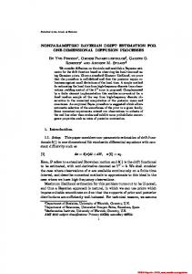
where mk,` and m ¯ k,` denote the number of links and nonlinks between nodes in component k and `, not counting any links from node n, and rn,` is the number of links from node n to any nodes in component `. In order to perform Gibbs sampling we can now simply consider each node in turn; for each partition (including a new, empty partition) compute the product of Eq. (33) and (34); normalize to yield a categorical distribution over partitions; and sample a new z¯n according to this distribution. The final algorithm is summarized in Fig. 5. The result after running the Gibbs sampler for 2T iterations is a set of samples of z¯, where usually the first half is discarded for burn in. This yields a final ensemble {¯ z (t) : t ∈ 1, . . . , T } approximately sampled from the posterior. 2) Computational complexity: In the algorithm outlined in Figure 5 it can be observed that there are two loops: One over the T simulated samples and one over the N nodes in the network. In each run of the inner loop, a node is assigned to a cluster by the Gibbs sampler. In the following we consider the number of clusters K a constant (although of course it will vary depending on the network data), and examine how the computational complexity of the algorithm depends on the number of nodes and edges in the network. In the code in Figure 5 the variables M0, M1 and m, which hold the counts of nonlinks, links, and nodes, are recomputed in each iteration. In a more sensible implementation, these quantities would be precomputed and efficiently updated during the Gibbs sampling.
CPU-time (seconds)
6
1
1
0.8
0.8
0.6
0.6
0.4
0.4
0.2
0.2
0 0 0.5 1 1.5 2 2.5 ×10³ Nodes
0 0 1 2 3 4 5 6 7 ×10³ Edges
Fig. 6. Experiment demonstrating that the computational complexity grows linear in both the number of nodes N and edges L for the IRM model. The graphs used in the experiments are generated with K = 5 communities of equal size and φ = φc /N where φc is kept constant in the experiments ensuring that the number of edges L grows linearly with the number of nodes N in the generated networks. The Gibbs sampler used in the experiment was implemented to pre-compute M0, M1 and m resulting in a computational complexity of O(L) for each iteration of the sampler. Given are the mean CPU-times in seconds for the sampler and standard deviation across T = 10 iterations when varying the number of nodes (N ) and edges (L) in the generated graphs.
Evaluating the probability of assigning a node to each cluster then requires the computation of the vector r which holds the count of links from node n to each of the clusters. The time complexity of this computation is on the order of the node degree. Looping over the nodes gives a total time complexity of O(L) where L is the number of edges in the graph. To calculate the probabilities of assigning the nodes to the clusters for all N Gibbs samples requires 2K 2 N evaluations of the (logarithm of the) Beta function so the time complexity of this computation is O(N ). As a result, since in general L > N , the total computational complexity of the Gibbs sampler for the IRM model is O(L). Figure 6 demonstrates that this linear scaling is observed in practice when analyzing networks of varying numbers of nodes and edges. For comparison, Monte Carlo maximum likelihood inference in exponential random graph model based on endogenous network statistics requires the simulation of random networks from the ERGM distribution, which is inherently an O(N 2 ) operation. We should note though, that in practice we would not expect the time complexity of the IRM to scale linearly in the number of edges, since the number of clusters most likely would increase with the size of the network and since the number of required iterations of the Gibbs sampler might also go up.
C. Checking model fit Once an approximation of the posterior distribution has been obtained, we wish to check the implications of the model. This can include computing the posterior distribution of important quantities of interest, evaluating how well the model fits the data, and making predictions about unobserved data. 1) Computing posterior quantities: Say we are interested in some function f (¯ z ) that depends on the model. We can now
7
function Z = irm(X,T,a,b,A) N = size(X,1); z = true(N,1); Z = cell(T,1); % Initialization for t = 1:T % For each Gibbs sweep for n = 1:N % For each node in the graph nn = [1:n-1 n+1:N]; % All indices except n K = size(z,2); % No. of components m = sum(z(nn,:))'; M = repmat(m,1,K); % No. of nodes in each component M1 = z(nn,:)'*X(nn,nn)*z(nn,:)- ... % No. of links between components diag(sum(X(nn,nn)*z(nn,:).*z(nn,:))/2); M0 = m*m'-diag(m.*(m+1)/2) - M1; % No. of non-links between components r = z(nn,:)'*X(nn,n); R = repmat(r,1,K); % No. of links from node n logP = sum([betaln(M1+R+a,M0+M-R+b)-betaln(M1+a,M0+b) ... % Log probability of n belonging betaln(r+a,m-r+b)-betaln(a,b)],1)' + log([m; A]); % to existing or new component P = exp(logP-max(logP)); % Convert from log probability i = find(rand r ij
k,`
�! + (γ si + ai ) + (υ tj + bj ) + c , (87) >
>
where r ij denotes a vector of various between node similarities, si and ti denotes vectors of features (i.e. sideinformation) for node i and j respectively. w, γ, υ are parameters specifying the effect of the side-information in predicting links and a, b specify node specific biases whereas c is a global offset that can be used to define the overall link density. This formulation is closely related to the way in which exogenous predictors are included in the exponential random graph model. These frameworks readily generalizes to the non-parametric latent class, feature, and hierarchical models described above and makes it possible to include all the available information when modeling complex networks. In particular including side information may improve the identification of latent structure [26], [58] as well as the prediction of links [34]. IV. O UTLOOK The non-parametric models for complex networks use latent variables to represent structure in networks. As such they can be considered extensions of the traditional exponential random graph models. The non-parametric models here provide a principled framework for inferring the number of latent classes, features, or levels of hierarchy using non-parametric distributions such as the Chinese restaurant process (CRP),
Indian buffet process (IBP) and Gibbs fragmentation trees (GFT). A benefit of these non-parametric models over traditional parametric models of networks is that they can adapt to the complexity of the networks by defining an adaptive parametrization that can account for the needed level of model complexity. In addition, the Bayesian modeling approach admits a principled framework for the statistical modeling of networks and enables to take parameter uncertainty into account. In particular, the Bayesian modeling approach defines a generative process for networks which in turn can be used to simulate graphs, validate the models ability to account for network structure and predict links [34], [38], [43] while Bayesian non-parametrics bring an efficient framework for the inevitable issue of model order selection. The non-parametric Bayesian modeling of complex networks have many important challenges that are yet to be addressed. Below we outline some of these major challenges to point out some avenues of future research. A. Scalability Many networks are very large and efficient algorithms for inference in these large systems of millions to billions of nodes and billions to trillions of links will pose important challenges for inferring the parameters of the models. Here it is our firm belief it will be very important to focus on models that grow in complexity by the number of links rather than the sizes of the networks as well as inference procedures that can exploit distributed computing. As such, models will have to be carefully designed in order to be scalable and parallelizable. While the latent class models described all scale by the number of links the LFRM and ILAM models explicitly have to account for both links and non-links which makes them scale poorly compared to the more restricted IMRM model. Thus, flexibility here comes at the price of scalability. In particular, existing models that are scalable do not include the modeling of side-information for the direct modeling of links. Thus, future work should focus on building flexible scalable models for networks. B. Structure emerging at multiple levels Network structure is widely believed to emerge at multiple scales [53], [44], [47], [50], [7], [48], [33], [19]. A limitation of latent class models are that they define a given level of resolution in which structure is inferred. Whereas latent feature models can generate features defining clusters at multiple scales [43] this property can be explicitly taken into account by the latent hierarchical models. An important future challenge will be to define models that can operate at multiple scales while efficiently accounting for prominent network structure by combining ideas from the latent hierarchical models with existing latent class and feature models. This includes hierarchical models that explicitly account for community structure and models that allow for the nodes to be part of multiple groups on multiple hierarchical levels. C. Temporal evolution Many networks are not static but evolve over time [39], [22], [51]. Rather than modeling snapshots of graphs as
16
independent, taking into account the timing in which links are generated, when nodes emerge and vanish etc. potentially brings important information about the structure in these systems. To formulate non-parametric Bayesian models that can model networks exhibiting time-varying complexity, such as clusters that emerge and disappear and hierarchies that expand and contract, poses an important future challenge for the modeling of these time evolving networks. D. Generic modeling tools As of today non-parametric Bayesian models for complex networks often have to be implemented more or less from scratch in order to accommodate the specific structure of the networks at hand. It will be very useful in the future to develop generic modeling tools in which general nonparametric Bayesian models can be specified including how parameters are tied, various distributions invoked, and sideinformation incorporated. Publicly available non-parametric Bayesian software tools for complex networks that can well accommodate the needs of researchers modeling complex networks will be essential for these models to fully meet their potentials and be adopted by the many different research communities that today use models and analysis of complex network as an indispensable tool. E. Testing efficiently multiple hypotheses Despite the very different origin of complex networks it is widely believed generic properties exist across the domains of these systems. What are the generic properties of networks and how can they be best modelled is an important open problem that is in need of being addressed. Non-parametric Bayesian modeling forms a framework for inferring structure across multiple hypothesis. For example, the IRM model itself encompasses the hypotheses of the Erd˝os-R´enyi random graph (an IRM with a single cluster) as well as the limit of the network itself (an IRM with a cluster for each node). Bayesian non-parametrics can here in general be used to infer structure across multiple hypotheses both including model order as in latent class models, feature representation as in the latent feature models, and types of hierarchies as in the latent hierarchical models. Non-parametric Bayesian models for complex networks is emerging as a prominent modeling tool that both provides a principled framework for model order selection as well as model validation. As the non-parametric Bayesian models also can give an interpretable account of otherwise complex systems it is our firm belief these models will become essential in order to deepen our understanding of the structure and function of the many networks that surrounds us. There is no doubt the future will bring many new non-parametric Baysian models for complex networks and that these models will find important new application domains. We hope this paper will facilitate researchers to tap into the power of Bayesian nonparametric modeling of complex networks as outlined in this paper to address the major challenges we face in our effort to understand and be able to predict the behaviors of the many complex systems we are an integral part of.
ACKNOWLEDGEMENTS This work is funded in part by The Lundbeck Foundation. R EFERENCES [1] E. Airoldi, D. Blei, S. Fienberg, and E. Xing, “Mixed membership stochastic blockmodels,” The Journal of Machine Learning Research, vol. 9, pp. 1981–2014, 2008. ´ ´ e de Prob[2] D. Aldous, “Exchangeability and related topics,” in Ecole d’Et´ abilit´es de Saint-Flour XIII–1983, ser. Lecture Notes in Mathematics. Springer, 1985, pp. 1–198. [3] K. Andersen, M. Mørup, H. Siebner, K. Madsen, and L. Hansen, “Identifying modular relations in complex brain networks,” IEEE International Workshop on Machine Learning for Signal Processing, 2012. [4] A. Barabasi and R. Albert, “Emergence of scaling in random networks,” Science, vol. 286, no. 5439, pp. 509–512, Oct. 1999. [5] D. Blei and M. Jordan, “Variational inference for Dirichlet process mixtures,” Bayesian Analysis, vol. 1, no. 1, pp. 121–144, 2006. [6] K. B¨orner, S. Sanyal, and A. Vespignani, “Network science,” Annual review of information science and technology, vol. 41, no. 1, pp. 537– 607, 2007. [7] A. Clauset, C. Moore, and M. Newman, “Hierarchical structure and the prediction of missing links in networks,” Nature, vol. 453, no. 7191, pp. 98–101, 2008. [8] N. R. C. Committee on Network Science for Future Army Applications, Network Science. The National Academies Press, 2005. [9] R. Cross and A. Parker, The Hidden Power of Social Networks. Harvard Business School Press, 2004. [10] V. Eguiluz, D. Chialvo, G. Cecchi, M. Baliki, and A. Apkarian, “Scalefree brain functional networks,” Phys Rev Lett., vol. 94, no. 1, p. 018102, 2005. [Online]. Available: http://arxiv.org/abs/cond-mat/0309092 [11] S. Fortunato, “Community detection in graphs,” Physics Reports, vol. 486, no. 3-5, pp. 75–174, 2010. [12] O. Frank and D. Strauss, “Markov graphs,” Journal of the American Statistical Association, pp. 832–842, 1986. [13] A. Gelman, J. Carlin, H. Stern, and D. Rubin, Bayesian Data Analysis. Chapman & Hall/CRC, 2004. [14] S. Gershman and D. Blei, “A tutorial on Bayesian nonparametric models,” Journal of Mathematical Psychology, vol. 56, no. 1, pp. 1–12, 2012. [Online]. Available: http://arxiv.org/abs/1106.2697 [15] P. Green and S. Richardson, “Modelling heterogeneity with and without the Dirichlet process,” Scandinavian Journal of Statistics, vol. 28, no. 2, pp. 355–375, 2001. [Online]. Available: http: //onlinelibrary.wiley.com/doi/10.1111/1467-9469.00242/abstract [16] T. Griffiths and Z. Ghahramani, “Infinite latent feature models and the indian buffet process,” in Advances in Neural Information Processing Systems, 2006, pp. 475–482. [17] ——, “The indian buffet process: An introduction and review,” Journal of Machine Learning Research, vol. 12, no. April, pp. 1185–1224, 2011. [Online]. Available: http://www.jmlr.org/papers/volume12/griffiths11a/ griffiths11a.pdf [18] T. Herlau, M. Mørup, M. Schmidt, and L. Hansen, “Dense relational modeling,” IEEE International Workshop on Machine Learning for Signal Processing, 2012. [19] ——, “Detecting hierarchical structure in networks,” Proceedings of Cognitive Information Processing, 2012. [20] P. Hoff, “Multiplicative latent factor models for description and prediction of social networks,” Computational & Mathematical Organization Theory, vol. 15, no. 4, pp. 261–272, 2009. [21] J. Hofman and C. Wiggins, “Bayesian approach to network modularity,” Physical Review Letters, vol. 100, no. 25, Jun. 2008. [22] K. Ishiguro, T. Iwata, N. Ueda, and J. Tenenbaum, “Dynamic infinite relational model for time-varying relational data analysis,” in Advances in Neural Information Processing Systems, 2010, pp. 919–927. [23] K. Ishiguro, N. Ueda, and H. Sawada, “Subset infinite relational models,” International Conference on Artificial Intelligence and Statistics, 2012. [24] S. Jain and R. Neal, “A split-merge Markov chain Monte Carlo procedure for the Dirichlet process mixture model,” Journal of Computational and Graphical Statistics, vol. 13, no. 1, pp. 158–182, 2004. [25] B. Karrer and M. Newman, “Stochastic blockmodels and community structure in networks,” Phys. Rev. E, vol. 83, 2011. [26] C. Kemp, J. Tenenbaum, T. Griffiths, T. Yamada, and N. Ueda, “Learning systems of concepts with an infinite relational model,” in Proceedings of the national conference on artificial intelligence, vol. 21. Menlo Park, CA; Cambridge, MA; London; AAAI Press; MIT Press; 1999, 2006, p. 381.
17
[27] D. Knowles and Z. Ghahramani, “Infinite sparse factor analysis and infinite independent components analysis,” Independent Component Analysis and Signal Separation, pp. 381–388, 2007. [28] P. Krivitsky and M. Handcock, “Fitting latent cluster models for networks with latentnet,” Journal of Statistical Software, vol. 24, no. 5, pp. 1–23, 5 2008. [Online]. Available: http://www.jstatsoft.org/v24/i05 [29] M. Kuhn, M. Campillos, I. Letunic, L. Jensen, and P. Bork, “A side effect resource to capture phenotypic effects of drugs,” Molecular systems biology, vol. 6, no. 1, 2010. [30] J. Leskovec, Dynamics of large networks. ProQuest, 2008. [31] P. McCullagh, J. Pitman, and M. Winkel, “Gibbs fragmentation trees,” Bernoulli, vol. 14, no. 4, pp. 988–1002, 2008. [32] E. Meeds, Z. Ghahramani, and S. Neal, R.M. Roweis, “Modeling dyadic data with binary latent factors,” in Advances in Neural Information Processing Systems, 2007, pp. 977–984. [33] D. Meunier, R. Lambiotte, and E. Bullmore, “Modular and hierarchically modular organization of brain networks.” Frontiers in neuroscience, vol. 4, 2010. [Online]. Available: http://dx.doi.org/10.3389/fnins.2010. 00200 [34] K. Miller, T. Griffiths, and M. Jordan, “Nonparametric latent feature models for link prediction,” in Advances in Neural Information Processing Systems, 2009, pp. 1276–1284. [35] M. Morris, M. Handcock, and D. Hunter, “Specification of exponentialfamily random graph models: Terms and computational aspects,” Journal of Statistical Software, vol. 24, no. 4, pp. 1–24, 5 2008. [Online]. Available: http://www.jstatsoft.org/v24/i04 [36] M. Mørup and M. Schmidt, “Bayesian community detection,” Neural Computation, vol. 24, no. 9, pp. 2434–2456, 2012. [37] M. Mørup, M. Schmidt, and L. Hansen, “Infinite multiple membership relational modeling for complex networks,” NIPS workshop on Networks across diciplines in theory and applications, 2010. [38] ——, “Infinite multiple membership relational modeling for complex networks,” IEEE International Workshop on Machine Learning for Signal Processing, 2011. [39] P. Mucha, T. Richardson, K. Macon, M. Porter, and J. Onnela, “Community structure in time-dependent, multiscale, and multiplex networks,” Science, vol. 328, no. 5980, pp. 876–878, 2010. [40] R. Neal, “Bayesian mixture modeling,” Maximum Entropy and Bayesian Methods: Proceedings of the 11th International Workshop on Maximum Entropy and Bayesian Methods of Statistical Analysis, pp. 197–211, 1992. [41] M. Newman, “Modularity and community structure in networks,” Proc. Natl. Acad. Sci., vol. 103, no. 23, pp. 8577–8582, 2006. [42] K. Nowicki and T. Snijders, “Estimation and prediction for stochastic blockstructures,” Journal of the American Statistical Association, vol. 96, no. 455, pp. 1077–1087, 2001. [43] K. Palla, D. Knowles, and Z. Ghahramani, “An infinite latent attribute model for network data,” International Conference on Machine Learning, 2012. [44] E. Ravasz, A. Somera, D. Mongru, Z. Oltvai, and A. Barab´asi, “Hierarchical organization of modularity in metabolic networks,” Science, vol. 297, no. 5586, pp. 1551–1555, 2002. [45] G. Robins, P. Pattison, Y. Kalish, and D. Lusher, “An introduction to exponential random graph (p*) models for social networks,” Social networks, vol. 29, no. 2, pp. 173–191, 2007. [46] G. Robins, T. Snijders, P. Wang, M. Handcock, and P. Pattison, “Recent developments in exponential random graph (p*) models for social networks,” Social Networks, vol. 29, no. 2, pp. 192–215, 2007. [47] D. Roy, C. Kemp, V. Mansinghka, and J. Tenenbaum, “Learning annotated hierarchies from relational data,” in Advances in Neural Information Processing Systems, 2007, p. 1185. [48] D. Roy and Y. Teh, “The mondrian process,” in Advances in Neural Information Processing Systems, 2009, pp. 1377–1384. [49] M. Rubinov and O. Sporns, “Complex network measures of brain connectivity: Uses and interpretations,” NeuroImage, vol. 52, no. 3, pp. 1059–1069, 2010. [50] M. Sales-Pardo, R. Guimera, A. Moreira, and L. Amaral, “Extracting the hierarchical organization of complex systems,” Proceedings of the National Academy of Sciences, vol. 104, no. 39, p. 15224, 2007. [51] P. Sarkar, D. Chakrabarti, and M. Jordan, “Nonparametric link prediction in dynamic networks,” ICML, 2012. [52] M. Schmidt, T. Herlau, and M. Mørup, “Nonparametric bayesian models of hierarchical structure in complex networks,” ArXiv, 2012. [53] H. Simon, “The architecture of complexity,” Proceedings of the American philosophical society, vol. 106, no. 6, pp. 467–482, 1962. [54] O. Sporns, Networks of the Brain. The MIT Press, 2010.
[55] U. von Luxburg, “A tutorial on spectral clustering,” Statistics and Computing, vol. 17, no. 4, pp. 395–416, 2007. [56] S. Wasserman and G. Robins, “An introduction to random graphs, dependence graphs, and p*,” Models and methods in social network analysis, pp. 148–161, 2005. [57] D. Watts and S. Strogatz, “Collective dynamics of ’small-world’ networks,” Nature, vol. 393, no. 6684, pp. 440–442, Jun. 1998. [58] Z. Xu, V. Tresp, K. Yu, and H. Kriegel, “Learning infinite hidden relational models,” Uncertainity in Artificial Intelligence, 2006. [59] W. Zachary, “An information flow model for conflict and fission in small groups,” Journal of anthropological research, pp. 452–473, 1977.