Numerical computation of equilibrium bid functions in a first-price ...

¢ ~ ExperimentalEconomics, 1 147-159 ( 1998) © 1998 Economic Science Association

Numerical Computation of Equilibrium Bid Functions in a First-Price Auction with Heterogeneous Risk Attitudes MARK V. VAN BOENING Department of Economics and Finance, University of Mississippi STEPHEN J. RASSENTI AND VERNONL. SMITH Economic Science Laboratory, 116 McClelland Hall, University of Arizona, Tucson, AZ 85721

Abstract

We use numerical methods to compute Nash equilibrium (NE) bid functionsfor four agents bidding in a first-price auction. Each bidder i is randomly assigned: r i ~ [0, rmax],where 1 -- ri is the Arrow-Pratt measure of constant relative risk aversion. Each ri is independently drawn from the cumulative distribution function q~(-), a beta distribution on [0, rmax]. For various values of the maximum propensity to seek risk, rmax,the expected value of any bidder's risk characteristic, E (ri), and the probability that any bidder is risk seeking, P (r i > 1 ), we determine the nonlinear characteristics of the (NE) bid functions. Keywords: auctions, equilibrium bidding, numerical analysis JEL Classification: D44

1.

Introduction

Equilibrium bidding theory in first-price auction with heterogeneous risk attitudes was developed initially in (Cox et al., 1982a) and further elaborated and generalized in (Cox et al., 1982b, 1988). Since the empirical bid functions reported in (Cox et al., 1988) showed a pronounced linear relationship between individual i's bid, bi, and the corresponding individual value, vi, much of the theoretical discussion has focused on the case in which agents are assumed to be constant relative risk averse in the monetary gains from bidding, with ri ~ [0, 1], where 1 - ri is the Arrow-Pratt measure of constant relative risk aversion. This case leads to what has become known as C R R A M the constant relative risk averse model of bidding. Even with C R R A M , however, the bid function is not linear over the entire domain of its support: the bid function is linear below a critical value, v*, unique to i, and has some unknown nonlinear shape that cannot be expressed in closed form for values above v*. This fact has been misunderstood and has led to erroneous conclusions (See Cox et al., 1992, pp. 1399-1400, and the references therein). In this paper we use numerical methods to explore the characteristics of the nonlinear upper portion of the bid function under various parametric assumptions about C R R A M ,

148

VAN BOENING, RASSENTI AND SMITH

including extensions of the interval over which ri is defined to allow for risk preferring agents, with ri E [0, rrnax], rmax = 2, 3. This results in graphical representations of CRRAM bid functions for these bench mark parameters. This work complements that of Cox and O axaca (1994a, 1994b) which explores empirically the extent of nonlinear bidding behavior in the experimental data on first-price auctions for the case ri E [0, 1].

2. Theory Consider a sealed-bid first-price auction with N = 4 bidders and Q = 1 item to be auctioned. The seller's reservation price is 0, so that no nonpositive bid can be a winning bid. Each bidder's monetary valuation vi, i = 1 to 4, for the item is independently drawn from the cumulative distribution function (cdf) H (v) on [0, Vm~x]. H(v) has a continuous probability density function (pdf) h(v) that is positive on (0, Vmax). Each bidder i knows vi, but only the distribution from which rivals' valuations are drawn. Assume that bidder i's preferences over income Yi can be represented by Ui (Yi) = (Yi)r~, w h e r e ri is the ith bidder's risk parameter and Ui (Yi) is normalized so that Ui (0) = 0. Each ri is independently drawn from cdf *(r) on [0, rn~x]; * (r) has a continuous pdf 4~(r) that is positive on (0, rm~x). Each bidder i knows ri, but only the distribution from which rivals' risk parameters are drawn. When 0 < ri < 1 then the ith bidder is risk averse, if ri = 1 then she is risk neutral, and if 1 < ri < rmax then she is risk preferring) Let G(bi) denote the probability that bi is the winning bid. Then the expected utility of bid bi is EUi(bi) = (vi - b i ) ~ "G(bi).

(1)

Assume that the ith bidder believes each rival will use a differentiable bid function b(v, r) which is strictly increasing in v with b(0, r) = 0. The first-order conditions for expected utility maximization yield 0

t

0

b p = v i - riG(b i ) / G (bi ).

(2)

For simplicity, the expression b(v, r) is used below to represent the unindexed equilibrium bid function generated by solving (2). Let the value b* be the maximum possible bid that can be made by the least risk averse (or most risk preferring) bidder in the population from which the N bidders are drawn. By ( 2 ) , b * = Vmax - rmaxG(b*)/G'(b*), and every bidder's maximum possible bid is at least b*. So in the region where b < b*, the probability that any one bidder using b(v, r) will bid less than or equal to amount b is given as F(b) =

(m~f'~dH(v)d'V(r); dO

dO

(3)

where Vhigh = b + rG(b)/G'(b) is the highest value, for a given r, that would generate a bid no greater than b.

149

N U M E R I C A L BID FUNCTIONS

For N = 4 and Q = 1, G(b) = F(b) 3, i.e., the probability that the three rivals will all bid less than b is given by the probability distribution of the third-order statistic for F(b). Cox, Smith, and Walker (1988) show that for N = 4, Q = 1, and H ( v ) = V/Vmax (i.e., h(v) is uniform [0, Vmax]), the noncooperative expected utility maximizing Nash equilibrium bid function is N-

1

b° - N - 1 + r i

Vi

--

3 3 + ri

1)i

forb ° < b* -

-

-

3

3 + rmax

Vmax.

(4)

Above b*, the Nash equilibrium bid function, when h(v) is Uniform [0, Vmax],cannot be expressed in closed form. Let rsmall = (Vmax- b) G'(b) / G (b) be the smallest risk coefficient, given a value Vmax,that would generate a bid no greater than b. Then the probability of a

bid less than or equal to b > b* can be written ag the sum of two integrals: F(b) =

dH(v) d ~ ( r ) + JO

,10

/r?/o

dH(v) d~p(r).

(5)

mall

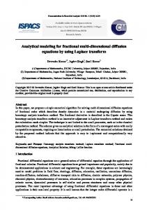
The two regions of integration in (5) are shown in the upper panel of figure 1. Note that for all b > b*, the function b(v, r) is not differentiable at r = (Vmax - b ) G ' ( b ) / G ( b ) . Consequently, there is a knot at b* separating the bid function into two segments. As shown in the lower panel, this has two important consequences for the Nash bid function of bidders with ri < rmax. First, the more risk averse the bidder (i.e., the closer ri is to 0), the smaller the support of the equilibrium strategy represented by (4). Second, the support decreases as rmax increases, since b* is inversely related to rmax. From (4), -3 Ob*/Ormax -- (3 + rmax)2 Vmax < 0.

(6)

Thus, a substantial portion of the support of the equilibrium strategy for any bidder may not be represented by (4) if the population includes risk preferring agents. For example, if rm~x = 2, then b* = .6Vmaxin (4) and figure 1. A detailed approach to solving for the nonlinear part of the bid function (5) as an initial value problem is given in Appendix.

3.

Numerical analysis

The solution to the initial value problem in Appendix is computed using the fourth-order Runge-Kutta method. 2 The resulting tables of F ( b ) and F'(b) are then used in (2) to calculate b(v, r) for b > b* (recall that G(b) = F(b)3). For simplicity, we normalize v so that Vmax= 1. 3.1.

Treatments

The solution of the initial value problem depends in part on assumptions about the risk preferences of bidders, as • (r), E ( r ) and rmax must be specified. Table 1 gives the equilibrium

VAN BOENING, RASSENTI AND SMITH

150

V

Vmax-

b>b*-

b*

)

) d"Cv)di'CrlI l l l } < ~ >

0

} d.¢v)dlCO F

(Vmax-b)G'(b)lG(b)

0

r max

r

b bmax--

b(v,r) for a bidder with r i < rmax

b =V/ii f

??

-"

i

., ," i

b=

~ y

r

N-l+r i

/ /

~

J

the least risk averse "bidder in the population

0

v max

V

Figure1. The effect of b on the Nash equilibriumbid function b(v, r). bid function under three different treatments where rmax, E(r), and the probability of risk preferring bidders P(r > l) are systematically varied. We utilize beta probability density functions (pdf) to characterize the distribution of risk preferences, as the shape and scale parameters can be manipulated to obtain a variety of distributions. By specifying E ( r ) , rmax and P(r > 1), a unique beta pdf ~b(r), 3 and thus the cumulative distribution function

151

NUMERICALBID FUNCTIONS Table 1. Numerical analysis treatments. rn~ax

b*

1 1 1 1 1 1

.75 .75 .75 .75 .75 .75

0.5 0.5 0.5 0.8 0.8 0.8

B1 B2 B3

2 2 2

.60 .60 .60

0.5 0.5 0.5

.05 .10 .20

beta(2.3,6.9) beta(l.3, 3.9) beta(0.4,1.2)

B4 B5 B6

2 2 2

.60 .60 .60

0.8 0.8 0.8

.05 .10 .20

beta(26.5,39.75) beta(16.0,24.0) beta(6.7,10.05)

3 3 3 3 3 3

.50 .50 .50 .50 .50 .50

0.5 0.5 0.5 0.8 0.8 0.8

.05 .10 .20 .05 .10 .20

beta(2.8,14.0) beta(1.5,7.5) beta(0.2,1.0) beta(33.6,92.4) beta(19.9,54.725) beta(7.9,21.725)

Distribution

E(r) P(r > 1)

~b(r)

Treatment 1 A1 A2 A3 A4 A5 A6

beta(0.5, 0.5) beta(1.0, 1.0) beta(4.0, 4.0) beta(2.0, 0.5) beta(6.0, 1.5) beta(16.0, 4.0)

D

Treatment 2

Treatment 3 C1 C2 C3 C4 C5 C6

Note: v normalized so that Vmax= 1. (cdf) • (r), is obtained. The parameters of the beta pdfs qb(r) are shown in the last column of Table 1.4 Under Treatment 1, all bidders are either risk averse or risk neutral, i.e., rmax = 1 so that P(r > 1) = 0. Treatments 2 and 3 each allow for risk preferring bidders in the population, as rmax = 2 and 3, respectively. (Recall that rmax also determines b*, the maximum bid by the least risk averse bidder in the population.) Under all three treatments, the average bidder is risk averse, i.e., E (r) < 1, but the mean varies between E (r) = 0.5 and E (r) = 0.8. Finally, under Treatments 2 and 3, rmax and E(r) are held constant while the percentage of the population that is risk preferring is systematically varied between 5%, 10% and 20%. 3.2.

Treatment I results

The six Treatment 1 beta probability density functions are shown in figure 2. With rmax = 1 and P(r > 1) = 0, a unique distribution is not obtained simply by specifying E(r) and the beta density can take on a wide variety of shapes. Distribution A1 is "U-shaped" and bimodal at 0 and 1, implying that bidders tend to be either extremely risk averse or risk neutral. Distribution A2 is uniform on [0, 1]. Distribution A3 is unimodal and symmetric

VAN BOENING, RASSENTI AND SMITH

152

f(r) B-

rmax=l bet..._.~a

E(r._.J

5-

A1

0.5

,-

A3 A4 A5

o.5 0.8 o.8

A6

/

_

~1

I \ /I / .. L I I

I

1

0

- 0.0

0.2

0.4

0.6

0.8

1.0

Figure 2. Treatment 1 beta probability density functions.

about its mean E(r) = 0.5, with very little chance of either extremely risk averse bidders or risk neutral bidders. The last three distributions all have E(r) = 0.8, but A4 has a mode of one, while A5 and A6 have modes of 0.91 and 0.83, respectively. Figure 3 shows our results 5 Each of the six panels displays computed bid functions under the given assumption about ¢(r). For example, bM(v, r) are our estimated bid functions when ~b(r)= beta(0.5, 0.5); see Table 1. Computed functions are shown for individual bidders with r = 0.2, 0.5 and 0.8. For comparison, the dashed lines in each panel are the linear extrapolations of the Nash bid function (4) above b*. The three left-hand panels show results when E(r) = 0.5, while the three right-hand panels show results when E(r) = 0.8. There are several regularities evident in figure 3. First, the computed bid functions are clearly nonlinear above b*, especially for very risk averse bidders. Our results indicate that the slope of the bid function decreases, but remains positive. Second, the shape of the bid function is not independent of ~b(r). For example, compare bA[ and bA3. Third, the shape of the bid function is not independent of E(r), i.e., compare the r = 0.2 computed functions in the left panels where E(r) = 0.5 with those in the right panels where E(r) = 0.8. Very risk averse bidders, r = 0.2, react strongly to increases in E(r). While the effect is not as strong for bidders with r = 0.8, it is in the same direction.

3.3.

Treatment 2 and Treatment 3 results

Figure 4 shows the beta distributions used in Treatments 2 and 3, which allow for risk preferring bidders (rmax = 2 and 3, respectively). Recall that an increase in rmax reduces b*, and thus reduces the support for the Nash bid function. Under both treatments, the first three

153

NUMERICAL BID FUNCTIONS

b ,oo~ o.95-~

b "=~ o.~

(v,r) ~m.,=1

bat

I

E(~)=o.~

i

.

bA4 (v,r) r,~,=l

~

~(0=o.8

."

.,

.L

0.90

/

e=lim area f~tnctiorl --

--

0.8

/

b=(N-1/l~l-l+r)v

.I /

o~

i

i'=O.2

~ ' ~

/

estimmted "~unctl0rt . b={N.1/N.I +r)v

0,8

0.00

//

+ .

/

z

~

b ~.co

085

0g0

0_~

rmax = I E(r)=0.5

/

o.9o

0.70

,1

estlme,ted ~netion --

--

b=(N-1/N-l+r)v

:','.::.',:'r~.

000

0.85

r=0.2

b i.oo.

hA5 (V,r)

o.s

rm~=l

0,~

/

r=0.5

estlm~ted function

- -

--

--

/

/" /

/

"

i" l"

1 .o

q

070

B

,

"

"

"

~

0,B0

0,85

.....

bA3 (v,r)

"

o.~5

rrn~ =1

0.70

0.75

b

'

. . . .

'

0.1110

-- --

-

0 ' 7 0

1.00

/

e~;Sraate~ furlc~ort

0.05

'

0.75 ~

b=(N-|s'~-l+~v

/

.... 0,75

0.80

1.oo~

bA6 (v,r)

o.~s~

rrnnx = 1

~

J'~ f:O.2

r=O.5

r=l.o

:

0.85

0.g0

0,95

E(r)=0,8

o.go

/

~

r=0.2 --

e"

- , -,

0.70

/"

/

/

b

E(r)=0.5

o.eo

. . . .

0.g5

b ~

/ /"

t" /

b=(N-J/N-l+r)v J

0,80

V 100

/

085

080

0,75

r=O.2

1" : ~

0,90

o.go

/ -/ ,t ~,*~/~ /

:::l'..:

0,75

E(r)=0.B

/

....

....

/

r=l.0

,::,:

~00

b A 2 (v,r)

o.0:

/

" " "

V 0,~

/.

/

r=o.8

r=t.0

0.75

/

/

/

/

"~ r=o.8

- " -

070

/

01~

~

eslamama lunc~tion

-- --

b:{N-1/'N=I+r}V

/

,"

/

t V 1.00

f

.~

./"

j-

r=0.B

+ 0.75 0,70 0,70

:-:-

t=L0

0"70

V 0,75

0,,8,0

0.85

0.~

0.95

t_O0

,

''" = ....

0.70

r=~,0 , .... 0.75

, .... 0.80

, .... 0.8~

, .... 0,9O

~ .... 0.~'~

;Y 1 .oo

Figure 3. Numerical estimation results from Treatment 1.

distributions each have E(r) = 0.5, while the last three each have E(r) = 0.8. As shown in Table 1, while holding E(r) constant, P(r > 1) is varied between 5%, 10% and 20%. Figure 5 shows our Treatment 2 results. Each of the six panels displays computed bid functions under the given assumption about ~b(r). For example, bB1 (v, r) are our computed bid functions when ~(r) = beta(2.3, 6.9); see Table 1. Computed functions are shown for individual bidders with r = 0.2, 0.5, 0.8, 1.0 and 1.5. For comparison, the dashed lines in

VAN BOENING, RASSENTI AND SMITH

154

f(r) 11t

Treatmentrmax =2 2

'

beta E(r) P(r>l) B1 0.5 .05

AB4

6

[_~

B2

0.5

.10

Ba 4 ,

~1 1 ~'~

B3

0.5

.20 .05

B4 0.8 B5 0.8

B1 /,,-~

O 0.0

0.2 0.4 0.6 0.8

1.0 1.2

1.4 1.6

.10

~ ' ' ' ~ ' i r 1.8 2,0 2 . 2 2 , 4 2 . 6 2.8 3 . 0

f(r) lo-

f~c4

Treatment 3

a-

lf~/ l\ 1

rmax =3 beta E(r) P(r>l)

4-

~s~ ~

2-

~. ~

051

~t

•,.,., 0.0

0.2 0.4 0.6 0.8

C3 0.5

.20

c4

.05

C5 08

.10

C6

.20

', ' , . , . , 1.0

1.2

1.4

0.8

0.8

,.,., 1.6

.

.,.,.,.,

1.8 2,0 2 . 2 2 . 4

2 , 6 2.8

r 3.0

Figure4. Treatments2 and 3 beta probabilitydensityfunctions. each panel are the linear extrapolations of the Nash bid function (4) above b*. The three left-hand panels show results when E(r)=0.5, while the three right-hand panels show results when E(r)=0.8. Comparison of bB1, bB2 and bB3, and comparison of bB4, bB5 and bB6 illustrates the effect of changing P(r > 1) while holding E(r) constant. Pairwise comparisons, e.g., bB 1with bB4, illustrate the effect of changing E (r) while holding P (r > 1) constant. Both E(r) and P(r > 1) affect the bid function. For example, compare bB1 with bB3, and compare bB1 with bB4. Our results indicate that the slope of the bid function decreases

155

NUMERICAL BID FUNCTIONS

b

bB1

1.901

1"°1 m=2 b

(v,r)

rmax= 2

0,95

0,95:

E(r)=0.5

0.90 !:

/ /

y ( r ~ l ) = os

.. 1

--

---

estirtmteded~n?ofunctlo~la f . j ~ . - -

b=(N-1/r4-1-er)v ~ -

I=0.5

~-

j~,

r=0.8 r=1.o

~

0.75:

E(r)=OS

•

,:o~

0,851: 0.80

b B4 (v,r)

0.70

/"

P(r>1)=.05

:

/

0.85!

/

-0`80:

eslirnetedfuncllon

/

/

i •

-- -- b = ( N - 1 / N - l + r/ ) v i

I r=02 r=0.5 ,=0.8

/ /f~"--/

0.70

r=15

0.65

1:2.0

0.80

V

0.55',..:

0.50 0.55

t

~=1.5 O.65

0.55 0`80 0.55 0.70 0,75 0.00 0`8~ O.gO 0.95 1.00

b

1`80t

b B2 (vr)

0.95t

rmax =2 E(r)=0.5

0.901

J

/ /~./.

estimated function -- -- b=~l-lJN-l+r)v

/~

/

r=0,2 r=0.5 r=0`8

/

o.781

0`80 i

bw

r=1`8

~r

r

2.0

o,5e i 0.55

0.50

0.05

0.70

0.75

b

b BS (v r)

o.95!

rmax =2 E(r)=O.5 P(r>1)=.20

1.1~ i

0.75 :

, ....

b B5 (v,r)

o.D5!

rmax =2

, ....

, ....

, ....

E(r)=O 8

o.oo 0.85: i 0`80 :

, ....

,V

/ "

/ /

P(r>l)=.10 -e~Smatedfunction -- -- b=(N-1/N-l+r)v

/

/

i

~

/

/ r=0.2 r=O 5 r=0:0

/

/

0,80

0.85

0.90

0.95

estimated function -- -- b=~N-1/N-1+r)v

°701

b*

,=1.5

°`8'i

+

,,0

0.00 i 0.5," 0.55

1.00

0.~0

0.55

b / / /

/

/

r=0.2 r=D.5

/ / //

/

t=0.8 r=~,0

--

078 0.80

0.70

0.65:

o.~

0`80:

0`90

0.55:,

D . 5 ~ ;

0`80

0.55

0.90

0.95

E(r)=O 8 P(r> 1) =.20

o~85:

o.7o!

0,75

1.oo

rmax =2

0`901

/ /

0.70

b 136(v r)

1.00 : 0.05 :

./ O.BO :

, ....

....

0.70 :

0.651:

, ....

b ~.oo~ :i

0.85::

o`8oi

, ....

0.55 0,60 0.65 0.70 0,75 0.80 O.B6 0.90 o.g5 tOO

/ /

P(r>l)=,lO

r=2.0

. . . . . . . . . . . . . . . .

/ ~ ,/

/

numedcal estimate -- b = [(N-1)/(N-I+r)]v

i /

/

/ i

t=02

"/

110 -

c=0.5 t=oa

/

b ~

0.55 0`80 0.55 0.70 0.75 0`80 0.85 0.00 0`95 1.00

r=1.5

I~" 4 ; .

,

t20 . . . .

i

.

l

I

. . . .

i

. . . .

i

. . . .

i

. . . .

0.55 0,60 0.55 0.7O 0.75 0.50 0.85

,

. . . .

0.90

,

. . . .

0.95

i

1.00

Figure5. Numericalestimationresults from Treatment2. for higher values of r, and this effect is strongest for very risk averse bidders. As in Treatment 1, when E(r) = 0 . 8 , the bid function for those bidders has a slope of almost 0 when v exceeds (approximately) 0.80. Also, as in Treatment 1, the increase in E(r) has a substantial impact on very risk averse bidders. However, if there is a relatively high probability of risk preferring bidders, i.e., P (r > 1) = . 2 0 , a similar effect is obtained even if E(r) = 0.5. That is, for bidders with r = 0.2, bB3 is more like bB4, bB5, or bB6 than b~1 or bB2. Bidders with r = 0.8 are relatively unaffected by changes in either E(r) or P(r > 1);

VAN BOENING, RASSENTI AND SMITH

156

the strongest effect is observed for bB3. Inspection of figure 4 reveals that under distribution B3, the majority of the population is quite risk averse, even though 20% of the population is risk preferring. This combination appears to result in further "shaving" of bids, relative to the extrapolated Nash bid line, even for (nearly) risk neutral bidders. Figure 6 shows our Treatment 3 results. In general, the increase in rmax does not appear to have a substantial effect, as the computed functions in figure 6 are very similar to those in figure 5. We were somewhat surprised by this result (recall Eq. (6)), but it may due to

b

b Cl (v,r)

1.00: 0.95i O.gO::

rm~=3 E(r) =0.5 P(r>l)=.05

0.¢L5 :0.80::

estimated

/ / /~...~.

r=o.2

function

r=o.8

0.75:: - - - - b = |(N 0.70::

r=l.0

1.00~o~5~-

bc4(v,r) rm=x=z

o~o~o.55~

E[r) =0.8 P(r>l) =.05

0.65 !

0.5O! b* t=2,0 O.~i 0.50 O.45:.. 0.4150.500.550.500.650.700.700.800.¢50.900.951.00

0.50 0.55

0.80 0.75 0.70 0.65

b c 2 (v,r) rma x =3

/

E(r)=0.5 P(r>l)=.lO

/ ...~

-estlrm~s69,.ruction -- -- b " [(

r=o.2 r=O,5

"~

~ r=O.8 r=l.0

Oo.:.. ..

r=0.5 .. , . ,

, , , V 0.45 0.50 0.55 0,60 0.65 0.70 0.75 0.80 0.85 0.9O 0.90 1,00

1.oob

0,50

~=00~

r=l.0

bW

r:2.o

. . . . . . . . . . . . . . . . .

r=3.0

0.45 : V 0.450.500.550.6O 0.550.70 O.750.800.850.900.951.00

=oo:b

b CS (v,r)

0.85

rmax03

0.00

E(r) = 0 . 8

o.8.~

P(r>l)=.lO

./

/ / /

0.8O ~ m eistectd _ functaon 0.75 -- -- b = |(N-1}/(N-1+r)}v

"r=o2 r=0.st=o'5 r=1.0

0.70

0.08

0.85 o.go 0.05 0.8O - -

/ / / r:-o.z

0.50~ - ectimatedfunc~Onlv~ 0.75 -- -- b = [(N-t)/(N-I+r) 0.70¢-

0.65 ::

.oo:b 0.88 o~O o.58

/ /

b C3 (v, r) rm~ = 3 E(r) =0.5 P(r>l)=.20 estimatedfunction

/ / /

/ /

t / r=0.2 / r=0.5

0"50i"550"80ii0"L5107'0~0"75 -- b~= [ON-1)/(N-t - +f)]v - "~ ~ P ' / ' ~ / * "/ " r=2.0r="lor=0"80

0.65 0.5O by¢ r=2.0 0.55 0.50 r=.3.0 0 . 4 5 ; : : ~ ' , ~ " :::::I V 0.45 0,50 0.55 0.60 0.55 0.70 0.75 0.50 0.85 0.90 0.00 1.00

~ b

bcs(v,r)

0.05 o.0o 0.85 O.85 ~ 0,70 -- --

rm¢x =3 E(r) =0.8 P(r>l)=.20

0.55 0.50

Figure 6. NumericalestimationresultsfromTreatment3.

v

0.50

0.60

0.45: " 0.45 0.50 0.55 0JB00.85 0.70 0.75 0.80 0.85 O.g0 0.95 1.00

estirnctsdfunction b = |(N-1)/(N-t+r)l

s / / / / / /r=O ~. ~ r=0.5 ~ r=0.5 r=l .o

b~

~1r . . . . . . . . . . . . . . . . .

r=2.o

r=3.0

o4, v 0.45 0 0 0 0.00 0 . ~ O.65 0.70 O.75 8.55 0.58 0 ~ 0 0.90 1.00

157

NUMERICAL BID FUNCTIONS

the fact for the beta distributions we chose, the shape of ~0(r) is not dramatically altered when E(r) and P(r > 1) are held constant while rmax is increased. For example, compare B1 and C1 in figure 4. 4.

Conclusions

We use numerical methods to compute the portion of the first-price auction equilibrium bid functions that cannot be expressed in closed form. We document the following: (1) the character of the concave nonlinearity in the bid function above b*; (2) the dependence of the bid function form above b* on assumptions about the parameters defining ~b(r), e.g., very risk averse bidders react strongly to increases in E(r); (3) for risk preferring bidders increases in P(r > 1), the probability mass on the risk preferring part of ~b(r), increases the curvature of the bid function above b*; and (4) the effect of rmax on the bid-function is relatively weak under all parameterizations explored. Of particular interest is that even when rmax = 3 , with only half the bid function below b*, the equilibrium bid functions are quasilinear over 75-80% of their range across all the q~(r) distributions we study. This demonstrates an unexpected robustness of the linear CRRAM model, and illuminates the empirical finding that nonlinear bidding is of minuscule proportions. Methodologically this exercise demonstrates the extreme limitations of Nash equilibrium theory for predicting behavior if one is restricted to models simple enough to yield closed form solutions. Even the simple first-price auction with non-risk neutral bidders is not generally tractable without numerical methods.

Appendix Consider the following initial value problem. For N = 4, G(b) = F(b) 3, and H(v) = V/Vmax,(5) can be expressed as

F(b) f F(b) = 1 + 3F'(b) Jo

3(~--b)r'(b) (3(Vmax--b)F'(b)~ r,b) rO'(r) dr - (Vmax- b) '~ \ ~ ]. (A1)

Multiplying by F'(b)/F(b), differentiating and applying Leibniz rule to the integral on the right-hand side of (A1), and then rearranging yields

F'(b) [ [F(b) --k (Vmax- b)F'(b)] 3 ( v ~ , ~ - b ) F ' ( b ) F"(b) = F(b----)"[ -FSgT i T (VT~ --b) O(a'v"~F((b~F (b))

t

1"

Letting Yl (b) = F(b) and Y2 = F'(b), this second-order equation can be transformed into a system of nonlinear first-order difference equations:

yt~(b) = Y2(b)

(A3)

VAN BOENING, RASSENTI AND SMITH

158

and

[Yl(b)

Y2(b)

+ (Vmax -

b ) Y 2 ( b ) ] ~ ( ~ )

-

Y2(b)

y~(b) . . . . Yl(b)

(A4)

W i t h H ( v ) = V/Vmax and G(b) = F ( b ) 3, for all b < b* Eq. (3) i m p l i e s that

~r

I~(-~ F(b*)

b,±r O(b*)

F(b*)

b* + ~ , , j ~ v - 7 ~ )

dH(v) d ~ (r) = --

dO

(A5) 1)max

dO

L e t t i n g 0 = 1 / E ( r ) and r e a r r a n g i n g w e get

F'(b*) = F(b*)/30(F(b*)vmax - b*),

(A6)

w h i c h b y i n s p e c t i o n yields a s i m p l e linear solution o f the f o r m k - b*. S o l v i n g for the u n d e t e r m i n e d coefficient k gives

30 + 1 ] b* =

F(b*) =

L30vr~xJ

30+1 0(3 + rmax) '

(A7)

and

F'(b*) =

30+1

.

(A8)

30 - Vmax T h e e x p r e s s i o n s (A3), (A4), (A7) a n d (A8) c o m p r i s e an initial value p r o b l e m in a s y s t e m o f n o n l i n e a r first-order differential equations. N u m e r i c a l m e t h o d s can b e u s e d to find F(b) a n d F'(b) for b > b*.

Notes 1. The Pratt-Arrow risk premium is positive, zero and negative, respectively. Also note that risk averse bidders exhibit constant relative risk aversion and decreasing absolute risk aversion. 2. Yakowitz and Szidarovszky (1989), pp. 369-390. 3. If x is a beta random variable on [0, 1], a beta random variable of the same shape on [a, b] can be obtained by the lransformation a + (b - a)x. See Law and Kelton (1991), pp. 338-339 and 404. 4. The reader will note that the cdf of a beta distribution also does not have a closed form solution. Consequently, each of the q~(r)'s were also numerically estimated (see Press et al., 1986). 5. The data from all three treatments are available on request.

NUMERICAL BID FUNCTIONS

159

References Cox, J.C. and Oaxaca, R. (1994a). "Inducing Risk Neutral Preferences: Further Analysis of the Data." Department of Economics, University of Arizona, Journal of Risk and Uncertainty, to appear. Cox, J.C. and Oaxaca, R. (1994b). "Is Bidding Behavior Consistent with Bidding Theory for Private Value Auctions" Department of Economics, University of Arizona, In R.M. Isaac (ed.), Research in Experimental Economics, vol. 6, to appear. Cox, J.C., Roberson, B., and Smith, V.L. (1982a). "Theory and Behavior of Single Object Auctions??' In Vernon L. Smith (ed.), Research in Experimental Economics, vol. 2. Greenwich, CT: JAI Press. Cox, J.C., Smith, V.L., and Walker, J.M. (1982b). "Auction Market Theory of H~t~rog~n~u~ [lidd~[~' Economic Letters. 9, 319-325. Cox, J.C., Smith, V.L., and Walker, J.M. (1988). "Theory and Individual Behavior in First-Price Auctions." Journal of Risk and Uncertainty. 1, 61-69. Cox, J.C., Smith, V.L., and Walker, J.M. (1992). "Theory and Misbehavior of First-Price Auctions: Comment?' American Economic Review. 82, 1392-1412. Law, A.M. and Kelton, W.D. (1991). Simulation Modeling and Analysis, 2nd ed. New York: McGraw-HilL Pearson, K. (ed.). (1934). Tables of the Incomplete Beta-Function. Cambridge: Cambridge University Press. Press, W.H., Flannery, B.P., Teukolsky, S.A., and Vetterling, W.T. (1986). Numerical Recipes, Cambridge: Cambridge University Press. Smith, V.L. and Walker, J.M. (1992). "Rewards, Experience and Decision Costs in First Price Auctions." Economic Inquiry, to appear. Yakowitz, S. and Szidarovszky, E (1989). An Introduction to Numerical Computations. New York: MacMillan Publishing Co.