Aug 20, 1999 - Ak = bBy ® bAx + bAy ® bBx. (2) where bA* and bB* are the one-dimensional stiffness and mass matrices associated with the respective spatial.
Numerical Simulation and Immersive Visualization of Hairpin Vortices H. M. Tufo,1 P. F. Fischer,2 M. E. Papka,2 K. Blom3 August 20, 1999 Abstract To better understand the vortex dynamics of coherent structures in turbulent and transitional boundary layers, we consider direct numerical simulation of the interaction between a �at-plate-boundary-layer �ow and an isolated hemispherical roughness element. Of principal interest is the evolution of hairpin vortices that form an interlacing pattern in the wake of the hemisphere, lift away from the wall, and are stretched by the shearing action of the boundary layer. Using animations of unsteady three-dimensional representations of this �ow, produced by the vtk toolkit and enhanced to operate in a CAVE virtual environment, we identify and study several key features in the evolution of this complex vortex topology not previously observed in other visualization formats.
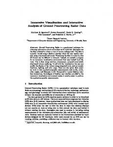
1 Introduction We present visualization results of numerically generated hairpin vortex formation and evolution in incompressible boundary layer �ows. At moderate �ow speeds, hairpin vortices provide an example of an observable, organized transition process from steady, two-dimensional laminar �ows to unsteady, threedimensional turbulent �ows. Consequently, hairpin vortices are of interest in the study of transitional and turbulent boundary layers, where they have been frequently observed experimentally. In this study, the hairpin vortices are generated in the wake of a hemispherical roughness element embedded in a �at-plate boundary layer, following closely the experiments of Acalar and Smith �1] and, to a lesser extent, those of Klebano� et al. �13]. Numerical studies of hairpin vortices have also been undertaken by Singer and his colleagues under slightly di�erent �ow conditions �2, 20, 21]. The basic �ow con�guration is shown in Fig. 1. A time-independent velocity pro�le is prescribed across the upstream entrance of the domain. Experimental observations �1] indicate that the �ow is symmetric about the plane y=0, so the �ow is computed only in the half-domain shown. At su ciently high nondimensional �ow speeds, or Reynolds numbers, the steady boundary layer region near the plate is destabilized by the hemisphere, resulting in periodic shedding of hairpin vortices in the wake. The simulation results are analyzed by using X-window-based software developed speci�cally for the numerical methods employed and using interactive software built on top of the \Visualization Toolkit" (vtk) to drive stereo visualization environments such as the CAVETM (Cave Automatic Virtual Environment) and ImmersaDeskTM . The resulting immersive visualization proceeds at a su ciently high frame rate that the Center on Astrophysical Thermonuclear Flashes, University of Chicago, Chicago, IL 60637. Mathematics and Computer Science Division, Argonne National Laboratory, Argonne, IL 60439. 3 Electrical and Computer Eng., Iowa State University, Ames, IA, 50011 1 2
1
Z Y
X
Figure 1: Computational domain showing inlet velocity pro�le, �at plate, hemisphere, and isolated hairpin vortex in hemisphere wake. For clarity, the vortex has been re�ected about the symmetry plane. hairpin evolution can be readily integrated by eye, thereby allowing one a comprehensive understanding of the dynamics of this complex �ow. The remainder of this paper is organized as follows. Section 2 provides a brief overview of the numerical method and speci�c �ow conditions considered. Section 3 describes the immersive visualization environment and software tools used. Section 4 presents a mixture of quantitative and qualitative visual results used to analyze this �ow. We close in Section 5 with a summary of our results.
2 Numerical Method and Flow Simulation This section describes the underlying discretizations, domain con�guration, and boundary conditions for the the hairpin vortex simulations.
2.1 Spectral Element Method The hairpin vortex simulation is based on numerical integration of the unsteady incompressible Navier-Stokes equations, @u + u u = 1 2u P + @t Re u = 0� r
;r
r
;r
coupled with appropriate boundary conditions on the velocity, u. Semi-implicit time stepping is employed in which the nonlinear convective terms are treated explicitly, while the viscous and pressure terms are treated implicitly. Spatial discretization is based on the spectral element method (SEM), which is a highorder weighted residual technique similar to the �nite element method. Within each element, basis functions are based on tensor-products of Nth-order Lagrange polynomials �5, 6, 14]. The nodes of the Lagrange polynomials are taken to be the Gauss-Lobatto-Legendre (GLL) quadrature points, so that high-order GLL quadrature can be substituted for the integrals required for the residual evaluation. The discretization is illustrated in Fig. 2, which shows a three-element mesh in lR2 with the GLL grid for the case N = 4. Also shown is the reference (r� s) coordinate system used for all function evaluations. Functions in the mapped 2
s
�1 y
6
�
�2
-
x
b
6 -
r
�3
Figure 2: Spectral element discretization in lR2 showing gll nodal lines for (K� N) = (3� 4). coordinates are of the form u(xk (r� s)) �k =
N N
XX
i=0 j =0
ukij hNi (r)hNj (s) �
(1)
where ukij is the nodal basis coe cient� hNi is the Lagrange polynomial of degree N based on the GLL quadrature points, �jN Nj=0 � and xk (r� s) is the coordinate mapping from the reference domain, �b := � 1� 1]d, to �k . The use of the GLL basis for the interpolants leads to e cient quadrature for the weighted residual schemes and greatly simpli�es operator evaluation in the case of deformed elements. For problems having smooth solutions, such as the incompressible Navier-Stokes equations, convergence is exponential in N, despite the fact that only C 0 continuity is enforced across elemental interfaces. The resulting (minimal) numerical dissipation and dispersion are ideal for transitional �ows of the type considered here, which can be very sensitive to such nonphysical e�ects. The rapid convergence is demonstrated in Table 1, which shows the computed growth rates of a small-amplitude Tollmien-Schlichting wave superimposed on plane Poiseuille channel �ow at Re = 7500, following �5, 16]. The amplitude of the perturbation is 10;5, so that the nonlinear Navier-Stokes results can be compared directly with linear theory to roughly �ve signi�cant digits. Three error measures are computed: error1 and error2 are the relative amplitude errors at the end of the �rst and second periods, respectively, and errorg is the error in the growth rate at a convective time of 50. From Table 1, it is clear that doubling the number of points in each spatial direction yields several orders of magnitude reduction in error, implying that just a small increase in resolution is required for very good accuracy. The signi�cance of this is underscored by the fact that, in three dimensions, the e�ect on the number of gridpoints scales as the cube of the relative savings in resolution. f
g
;
Table 1: Spatial convergence, O-S problem: K = 15� �t = :003125 N E(t1 ) error1 E(t2 ) error2 errorg 7 1.11498657 0.003963 1.21465285 0.037396 0.313602 9 1.11519192 0.003758 1.24838788 0.003661 0.001820 11 1.11910382 0.000153 1.25303597 0.000986 0.004407 13 1.11896714 0.000016 1.25205855 0.000009 0.000097 15 1.11895646 0.000006 1.25206398 0.000014 0.000041 3
2.1.1 Time Advancement The Navier-Stokes time advancement is based on the second-order operator splitting methods developed in �15]. The convective term is expressed as a material derivative, and the resultant form is discretized via a stable second-order backward di�erence formula: u~ n;2 4~un;1 + 3un = S(un) � 2�t n where S(u ) is the linear symmetric Stokes problem to be solved implicitly, and u~ n;q is the velocity �eld at time step n q computed as the explicit solution to a pure convection problem. The subintegration of the convection term permits values of �t corresponding to convective CFL numbers of 2{5, thus signi�cantly reducing the number of (expensive) Stokes solves. The Stokes problem is of the form ;
;
"
H D
;
DT
#�
un
!
�
= Bf 0
!
pn 0 and is also treated by second-order splitting, resulting in subproblems of the form ;
Huni = f i � for the velocity components (i = 1� : : :� 3), and Epn = g n � for the pressure. Here, H is a diagonally dominant Helmholtz operator representing the parabolic component of the momentum equations and is readily treated via Jacobi-preconditioned conjugate gradients� E := DB;1DT is the Stokes Schur complement governing the pressure� and B is the (diagonal) mass matrix in the velocity space. E is a consistent Poisson operator and is e�ectively preconditioned by using the overlapping additive Schwarz procedure of Dryja and Widlund �4]. Further details of the discretization and solvers may be found in �5, 6].
2.1.2 Spectral Element Operators The computational e ciency of spectral element methods derives from their tensor-product basis. To illustrate, we express the sti�ness matrix for an undeformed element k in lR2 as a sum of tensor products of one-dimensional operators, Ak = Bby Abx + Aby Bbx � �
�
(2)
where Ab� and Bb� are the one-dimensional sti�ness and mass matrices associated with the respective spatial dimensions. If uk = ukij is the matrix of nodal values on element k, then a typical matrix-vector product required of an iterative solver takes the form (Ak uk )lm = =
N N
XX
(Bby mj Abx li ukij + Aby mj Bbx li ukij )
i=0 j =0 Abx uk BbyT
+ Bbx uk AbTy :
The latter form illustrates how the tensor-product basis leads to matrix-vector products (Au) being recast as matrix-matrix products, a feature central to the e ciency of spectral element methods. Similar forms result for other operators and for complex geometries. 4
The parallel implementation follows a standard message-passing-based single-program-multiple-data (SPMD) model �9] in which contiguous groups of elements are distributed to processors. Since iterative solvers are used, the principal communication kernel is the gather-scatter operation required for the residual vector assembly procedure. Because data is always stored on an element-by-element basis, the gather-scatter procedure required for residual evaluation is combined into a single communication phase wherein shared nodal values are exchanged and summed. This is a single local-to-local transformation, rather than separate gather and scatter phases common to many �nite element implementations. The gather-scatter operation is implemented by using a stand-alone MPI/NX-based message-passing utility that supports a vector mode for problems having multiple degrees of freedom per vertex as well as a general set of commutative/associative operations �23]. The easy-to-use interface requires only two calls:
handle = gs-init(global-node-numbers,n), and
ierr = gs-op(u,op,handle),
where global-node-numbers() associates the n local values contained in the vector u() with their global counterparts, and op denotes the reduction operation performed on shared elements of u(). Communication overhead is further reduced through use of a recursive spectral bisection based element partitioning scheme to minimize the number of vertices shared among processors �18]. The spectral element code runs on a number of distributed-memory platforms, including the Intel Paragon, Cray T3E-600, SGI Origin 2000 and IBM SP. Simulations of the hairpin vortex problem have been run on 2048 333 MHz nodes of ASCI-Red in both in single- and dual-processor mode, with sustained performance of 319 GF being achieved for the latter �22].
2.2 Flow Simulation For the hairpin vortex simulations, we considered several meshes and computational domains to test grid and domain independence, with our two primary production meshes having K = 1021 and K = 1535 spectral elements. All of the meshes tested have a unit-radius hemisphere located with its center at (x� y� z) = (0� 0� :1). A short cylinder of height dz = :1 connects the hemisphere to the �at plate, which is located at z = 0. The cylinder was added so that a thin layer of elements could be placed near the plate to ensure adequate resolution of the boundary layer. The resultant 10% increase in the height of the hemisphere closely corresponds to height increases resulting from glue used to fasten the hemispheres in the experiments of Klebano� et al. �13]. We consider a Reynolds number range of ReR := UR=� = 450{850, where U is the free-stream velocity, R is the hemisphere radius, and � is the kinematic viscosity of the �uid. Flow is in the positive x direction with incoming �ow u = (uB (y)� 0� 0), where uB (y) represents a Blasius pro�le with �99 = 1:2R. The in�ow boundary is located at x = 8:4 for the K = 1021 mesh and at x = 10:0 for the K = 1535 mesh. To reduce the computational burden, we impose re�ection symmetry about the y-plane. Homogeneous Neumann boundary conditions are prescribed for the velocity at the outlet, located at x = 30. The upper boundary and the right boundary are also taken to be symmetry planes, corresponding to stress-free boundary conditions. These are located at z = 6:5 and y = 6:4 for K = 1021 and z = 8:0 and y = 8:4 for K = 1535. We note that, in addition to having di�erent size domains and number of elements, the two meshes have di�erent transitions between spherical and rectangular elements and between the in�ow boundary and hemisphere, with the K = 1535 mesh having a smoother transition for both. To transition between Reynolds numbers, we employ a sine ramp, Re(t) = Rei + (Ref Rei ) sin(gt), where Rei is the initial Reynolds number, Ref is the �nal Reynolds number, and g is the growth rate, typically set such that duration of the ramp is 40{80 convective time units. Figure 3a shows the pressure trace at x = (2:4� 0:0� 1:2) for an 80 time unit transition between Reynolds number 675 and 700. Once ;
;
;
;
;
;
;
5
-0.010
0.225
-0.015
0.220
-0.020
0.215
-0.025
0.210
-0.030
0.205 Strouhal Number
Pressure
0.230
-0.035 -0.040 -0.045
0.200 0.195 0.190
-0.050
0.185
-0.055
0.180
(a)
-0.060
K=1021
(b)
0.175
-0.065
0.170 0
50
100
150
200
K=1535 450
Time
500
550
600
650
Reynolds Number
Figure 3: (a) Transition from Re =675 to 700. (b) Strouhal number versus Reynolds number for the K = 1021 and K = 1535 meshes. the transition has been made, the �ow is driven until it settles into a steady periodic state. Of particular interest in these simulations is determination of the Strouhal number, S = fk=Uk , where f is the shedding frequency, k = 1:1 is the total height of the roughness element, and Uk is the tip velocity without the hemisphere present. Uk is calculated from a two-dimensional channel �ow simulation on a domain identical in dimension to the hemisphere symmetry plane (centerplane) but without the hemisphere. The frequency, f, is determined from history plots similar to Fig. 3a. Strouhal numbers for the K = 1021 and 1535 meshes are shown in Fig. 3b. For this study 3 N 15, with the maximum N considered for Reynolds number 450 being 9 and for Reynolds number 700 being 15. We note that the maximum discrepancy between the two meshes is less than 2% over the range of Reynolds numbers considered here and that spatial and temporal convergence checks were performed at several Reynolds numbers to verify convergence. We further note that our Strouhal numbers compare favorably to those in �1] and �13]. �
�
3 Visualization System The visualization of the spectral element data is addressed through a multistage process. The �rst step uses a menu-driven X-window-based postprocessor developed speci�cally for spectral elements. It exploits the full accuracy of the high-order Lagrangian basis (1) when interpolating o�-grid point values or computing derived quantities such as velocity gradients or vorticity. In addition, the postprocessor can map spectral element data onto unstructured hexahedral meshes of arbitrary density. This data is then processed for use in a second visualization package designed for immersive visualization of the general mesh data. The primary components of this second mode are built using the vtk library, which is an open-source software system for visualization that provides a high-level abstraction for constructing scienti�c visualization applications �19], and the CAVE library, which enables projection and exploration of immersive stereo images �3]. An overview of the entire visualization process is outlined in Fig. 4. 6
700
�� � � '$'$�� '$ �� �� �� �� &%&%���� ��&%
SEM -
�d
- vol -
srf1
srf2
srf3
srf4
- CAVE - mac - rib - BMRT 6
tif
Figure 4: Visualization process: SEM produces numerical output (�d), which is translated by the Xpostprocessor into vtk unstructured cell format (vol). These are processed into individual polygonal datasets (srf), representing isosurfaces of the vortex �eld at distinct threshold values, �, or at di�erent times. This data is then viewed interactively at low resolution in the CAVE, where camera paths are captured. The output (cam) is combined with (srf) to produce rib �les (rib). These are processed by the Blue Moon Rendering Tools (BMRT) to yield the �nal high-resolution output (tif).
3.1 Vortex Identi�cation Vortex identi�cation starts in the postprocessing phase and is based on the �2 method of Jeong and Hussain �10]. Identi�cation of a vortex in viscous �ows is challenging because the classic rules governing vortex dynamics generally apply only in the inviscid limit. In boundary layer �ows, viscosity is non-negligible, and standard approaches such as integrating vortex lines or using pressure minima or vorticity maxima can lead to improper vortex identi�cation. Jeong and Hussain have established a robust criterion for the identi�cation of vortex (or coherent) structures in viscous �ows based on the eigenvalues of the symmetric 3 3 tensor �
Mij := where
�
3 X ;
k=1
�
�ik �kj + Sik S kj �
!
(3)
�
!
@ui + @uj @ui @uj �ij := 21 @x Sij := 21 @x (4) @x @xi j i j represent the symmetric and antisymmetric components of the velocity gradient tensor, u. To minimize noise, the gradients are computed using the original polynomial description of the data, that is, by di�erentiating (1). Given the three (real) eigenvalues of M at each grid point, a vortex core is identi�ed as any contiguous region having two negative eigenvalues. If the eigenvalues are sorted such that �1 �2 �3, then any region for which �2 < 0 corresponds to a vortex core. One advantage of this approach is that vortices can be identi�ed as isosurfaces of a well-de�ned scalar �eld. Moreover, the criterion �2 (x) < 0 is scale invariant, so there is in principle no ambiguity in selecting which isosurface value to render. In practice, one usually biases the isosurface to a value that is below zero by a small fraction of the full dynamic range in order to avoid noise in regions where the velocity is close to zero. ;
r
�
�
3.2 Isosurface Extraction and Immersive Visualization To develop an unsteady immersive rendering of the vortex evolution, we begin with a set of full-volume dumps of the primitive variables (u� v� w� p) at a selected number of time steps (typ. 150) covering one period of the vortex shedding cycle. For each time step, we compute �2 at each grid point with the X-window based postprocessor. The high-order accuracy of the spectral element basis (1) is essential for this step. The resultant scalar �eld is then interpolated onto an unstructured hexahedral mesh along with the pressure. This volume of data is then passed to a surface stripper (built on top of vtk) to extract isosurfaces at a given 7
threshold, �, and produce a set of triangles corresponding to �2 = �. Typically, 2 � 1, out of a range of � 30� 40]. Visualization within the CAVE environment requires real-time response, and, because of the time required to generate isosurfaces, interactive generation of the surfaces is impossible. Figure 5 plots the average time required for the generation of an individual isosurface at a given threshold versus Reynolds number. The rise in time re�ects the increasing complexity of the �ow �eld with increasing Re. In addition to isosurface extraction, smoothing and triangulation algorithms are applied as part of the visualization pipeline to improve performance in the CAVE. The resulting surface �les are saved to disk in the vtk polydata format. This format contains all the information necessary to construct the geometric representation of the �2 isosurfaces with corresponding pressures at each vertex. For immersive visualization, the surface �les are loaded into another vtk-based application that is built on top of the CAVE library and is designed to run on all members of the CAVE family of display technology, including the ImmersaDesk. (The vtk classes for renderer and renderwindow have been extended to operate within the CAVE �7].) The CAVE is a 100 100 100 cube of rear-projected screens, illustrated in Fig. 5 (right), which allows the user to rapidly explore data from a number of di�erent viewing angles. The ImmersaDesk is single 50 rear-projected screen. Both are capable of displaying immersive stereo images. The immersive application makes full use of the CAVE library's rich set of tools that enable users to explore and interrogate individual surface �les, as well as a composited series of surface �les for time- or parameter-dependent data. For the Re = 700 surface �les a rate of 15 frames per second is achieved, which is more than su cient to produce a realistic sense of motion to the user. Control over viewing location, frame rate, and playback are provided by the combination of a navigational wand and virtual menu. In addition, users can de�ne a color table to map other scalars onto the �2 isosurfaces. At present, only the pressure is mapped. Within the immersive environment it is also possible to generate high-quality renderings of the surface data. The user can navigate to points of interest within the data set and take virtual snapshots or virtual movies of the experience, capturing the needed information for high-resolution rendering. This is done either ;
�
� ;
;
�
�
400
350
Time(s)
300
250
200
150
100 450
500
550 600 Reynolds Number
650
700
Figure 5: Two stages in the vizualization process. Isosurfaces for a series of images are precalculated o�-line. (Average calculation times versus Reynolds number are shown on the left.) Precomputed isosurfaces are then rendered at 15 frames per second in the CAVE (right) allowing interactive navigation of unsteady surface data and selection of speci�c views for high-resolution rendering. 8
by immediately generating a RenderMan RIB �le using a class provided within vtk for a snapshot, or by capturing the camera position and orientation information in virtual movie mode to allow o�-line rendering. (Virtual movie mode requires an additional o"ine step for generating the RIB �les, because the size of the �les would interfere with the required real-time response of the virtual environment.) Once the RIB �les are created, they are processed by using Blue Moon Rendering Tools (BMRT), a freely available collection of rendering tools that adhere to the RenderMan interface standard �8]. BMRT enables users to capture points of interest from within the data set in a high-quality format suitable for publication or videotape.
4 Results To put the dynamic results into perspective, we begin with a series of two-dimensional plots in the symmetry plane, y = 0. Figure 6 shows the results of a simulation at Re = 700 using 1021 elements of order N = 11. Time-averaged velocity pro�les are shown in (a), and corresponding rms values, urms :=< u02 > 21 , are shown in (b). Here u0 := u < u > is the �uctuating component of u, and < : > denotes a single-period time average. The pro�les have maximum values of 1.075 and 0.282 for u and urms , respectively. We see in (a) the Blasius pro�le at the inlet, the separated and recirculating wake region at x = 2, followed by a gradual recovery until the outlet, where the mean velocity pro�le is fuller than the in�ow pro�le. From the rms pro�les (b), it is clear that the �ow upstream of the hemisphere is essentially steady. The immediate wake region at x = 2 exhibits remarkably little unsteadiness. The passage of the hairpin vortices is evidenced by the strong rms �uctuations in the wake region, which also reveal the lifting of the vortices away from the plate. Further downstream, there is a signi�cant growth in activity near the wall, as can be seen by the peak in the rms pro�le at the outlet. To indicate the structure of individual hairpin vortices at a �xed instance, we present contours of several quantities in Fig. 6 (c{e). Pressure contours are shown in (c). The vortex cores are readily identi�ed by the low-pressure zones, shown in bold. Contours of spanwise vorticity (d) also show the hairpin vortices and, in particular, the movement of the heads and tips away from the plate. Finally, (e) shows contours of �2 � 30� 0], revealing the intersection of the vortex tips with the symmetry plane and the presence of a steady horseshoe vortex at the base of the hemisphere near x = 1: Results for Re = 450 are shown in Fig. 7. This is just above the critical Reynolds number at which the �ow transitions from a steady to a steady-periodic state. In contrast to the Re = 700 case, the wake de�cit in the symmetry plane pro�le (a) is very pronounced, even 30 radii downstream of the hemisphere. The rms pro�les (b) grow with increasing x, although the peak rms value of .063 is a fraction of that for the Re = 700 case. The shear layer observed in (a) indicates that the growth in rms values in (b) can be interpreted as the onset of a Kelvin-Helmholtz instability: slight oscillations in the wall-normal velocity component translate into signi�cant u0 �uctuations in the shear-layer region where @u @z is large. The oscillations and wave like nature of the �ow are quite evident in the contour plot of spanwise vorticity, shown at a �xed instant in the shedding cycle in (c). While the views in Figs. 6 and 7 provide a fair amount of information about the hairpin vortex evolution, they fail to reveal any three-dimensional details. To see these, we rely on output from the visualization process described in Section 3. Figures 8 and 9 show �2 = 1 isosurfaces for Re = 700. We observe several vortex features, some of which we had not identi�ed prior to viewing the unsteady animation in an immersive environment. Figure 8 shows the classic horseshoe vortex (a) upstream of the hemisphere, which is also commonly found upstream of end-mounted cylinders (as evidenced by snowdrift patterns at the bases of trees and telephone poles). Moving downstream, we see the interlacing of the hairpin vortex tails (b), as observed by Acalar and Smith �1]� the hairpin head (c)� and a vortex \bridge" (d), which is a common form ;
2
;
;
;
9
(a)
(b)
(c)
(d)
(e)
Figure 6: Symmetry plane data for Re = 700, K = 1021, N = 11 (a{b), and N = 13 (c{e): (a) mean velocity pro�les, < u >� (b) rms velocity < u02 > 21 � (c) pressure contours � (d) spanwise vorticity, !y � (e) contours of �2 < 0.
10
(a)
(b)
(c)
Figure 7: Symmetry plane data for Re = 450, K = 1535, N = 9: (a) mean velocity pro�les, < u >� (b) rms velocity < u02 > 12 � (c) spanwise vorticity, !y .
� � � �
�
@ I @
(a)
(b)
A K A A A A
(c)
� � � �
� �
�
(d)
Figure 8: Key vortex structures at Re = 700: standing horseshoe vortex (a), interlaced tails (b), hairpin head (c), and bridge (d). Contours mapped onto �2 = 1 surface represent pressure (light=high, dark=low). Shadows on the plate provide additional perspective information. ;
of vortex reconnection in viscous �ows �11, 12, 17, 24]. Acalar and Smith �1] note that the bridge-head structure eventually separates from the hairpin and lifts o� as a separate vortex ring. At this Reynolds number the ring is so quickly dissipated by viscosity that the lifto� is not pronounced. Because the bridge is quite thin and rather short lived, signi�cant resolution in space and time is required to see it. We carefully chose the frame in order to present the bridge here. However, initial detection of the bridge and other similar unanticipated structures requires observation of a sequence of images from many viewing angles. Another structure detected as a result of such interactive viewing is shown in Fig. 9. The \spikes" seen jutting from the interior of the hairpin loop are readily visible in most of the higher Reynolds 11
MBB
B B
B B
B B B
AA K
A
B B
spikes
A A A
A
tails
Figure 9: View showing distinction between \spikes" and tails of preceding vortex. number computations. They appear at just about the time that the tails of the preceding vortex disappear as a result of stretching-induced dissipation. Initially, we believed the spikes were remnants of the dissipating tails. However, careful observation of the animation revealed that the spikes and tails brie�y appear at the same time, indicating that they are not part of the same vortex structure. Downstream views of the head-spike structure seem to indicate that the spike formation is induced by the close proximity of the tails to the head, as seen in Fig. 8b. A comparison between the hairpin vortices at Re = 550 and 700 is shown in Fig. 10. Few structural di�erences are seen over this range of Reynolds numbers. However, there is a noticeable di�erence in the distance that separates the successive hairpins, with shorter distances for Re = 700 corresponding to a higher Strouhal number (cf. Fig. 3). In addition, the Re = 700 case shows stronger evidence of tail-tail interlacing and the presence of a second horseshoe vortex upstream of the hemisphere. We close this section with recently obtained results at Re = 850, shown in Fig. 11. The images reveal a cascade of vortices just a few diameters downstream of the hemisphere. At lower Reynolds numbers these vortices are not strong enough to yield the clearly de�ned structures that are present here. Clearly visible at this elevated Reynolds number are secondary vortices on either side of the hairpin, seen at the midpoint in the planform view. In addition, the lifto� of the hairpin head as a ring-vortex can be seen near the out�ow in the pro�le view. The pro�le also shows the general inclination of the vortices, rising from the wall and moving downstream, commonly observed in turbulent boundary layers.
5 Discussion and Conclusion We have examined the structure of hairpin vortices in the near wake region of a hemispherical roughness element at ReR = 700 using spectral element simulations coupled with interactive immersive visualization. This is part of a wider investigation, with Reynolds numbers ranging from 450 (just above transition) to 1200, into the role hairpin vortices play in the transition between laminar and turbulent �ow. We have shown excellent agreement between simulation and experimental data with regard to shedding frequency and clear identi�cation of the principal features of the primary hairpin vortex and its evolution. We found that the combination of immersion and motion played a key role in the assimilation, integration, and understanding of this data set and believe that immersive visualization tools, such as those developed here, will be essen12
(a)
(b)
(c)
(d)
Figure 10: Comparison pro�le views of hairpin vortices at Re = 550 (a) and Re = 700 (b), and planform views at Re = 550 (c) and Re = 700 (d). 13
Figure 11: Re = 850 pro�le (top) and planform (bottom) views of �2 = 1:1 isosurfaces for the full computational domain. ;
tial tools for future investigation of �ows where coherent structures play a key role in �ow transition and development. Further investigation is required into the nature of the secondary vortices that develop immediately downstream of the recirculation zone. Acalar and Smith observed two types of secondary vortices. The �rst formed in the wake of the hairpin and was entirely contained between the legs. It is an open question as to whether the bridge we observed corresponds to this structure and whether this is an example of classic vortex reconnection via bridging �12]. The second is a pair of vortices that form several diameters downstream of the hemisphere on either side of the primary hairpin vortex. We do indeed see the formation of such structures, which become more pronounced in recent calculations at higher Reynolds numbers. Singer and Joslin have shown that a cascade of such hairpins ultimately evolves into a turbulent spot �21]. Their calculations were in a plane channel, which allowed them to track the (isolated) vortex as it moved downstream, resulting in considerable computational savings. A similar approach could be used here, exploiting the temporal periodicity of the solution to provide a well-de�ned in�ow boundary condition. It is clear that straightforward calculation of spatially developing �ows from transition to turbulence in inhomogeneous geometries will require a signi�cant increase in resolution to capture the range of scales present in both the solution and the geometry. Exploration of extremely large data sets is di cult even with today's state-of-the-art visualization tools. For example, to store the primitive variables (u� v� w� p) for a 150-frame \movie" requires 5{20 GB. Since we are interested in determining how vortex topology varies with Reynolds number, we anticipate having tens to hundreds of such \movies" in our database. There is a consequent need for advanced technology to archive, manipulate, and explore data sets in excess of a terabyte. We are currently working on methods that facilitate such investigation. One promising path is to use subsampled or lower-resolution data sets for preliminary investigation and to record areas or paths where 14
high-resolution images are desired. These images can then be computed o"ine at full data set resolutions. We are developing this and other visualization software technology, such as automatic feature detection and tracking, to assist in the interrogation of large data sets such as considered here.
Acknowledgments This work was supported by the Mathematical, Information, and Computational Sciences Division subprogram of the O ce of Advanced Scienti�c Computing Research, U.S. Department of Energy, under Contract W-31-109-Eng-38, and by the Department of Energy under Grant No. B341495 to the Center on Astrophysical Thermonuclear Flashes at the University of Chicago.
References
�1] M. S. Acalar and C. R. Smith, \A study of hairpin vortices in a laminar boundary layer: Part 1, hairpin vortices generated by a hemisphere protuberance", J. Fluid Mech., 175, pp. 1{41 (1987). �2] D. C. Banks, T. Crockett, R. D. Joslin, B. A. Singer, \Parallel Rendering of Complex Vortical Flows", http://www.icase.edu/docs/hilites/banks/parallelRend.html. �3] C. Cruz-Neira, D. J. Sandin and T. A. DeFanti, \Surround-screen projection-based virtual reality: The design and implementation of the CAVETM ", Computer Graphics (Proceedings of SIGGRAPH '93), ACM SIGGRAPH, August, pp. 135{142 (1993). �4] M. Dryja and O. B. Widlund, \An additive variant of the Schwarz alternating method for the case of many subregions", Technical Rep. 339, Dept. Comp. Sci., Courant Inst., NYU (1987). �5] P. F. Fischer, \An overlapping Schwarz method for spectral element solution of the incompressible Navier-Stokes equations", J. Comp. Phys., 133, pp. 84{101 (1997). �6] P. F. Fischer, N. I. Miller, and H. M. Tufo, \An overlapping Schwarz method for spectral element simulation of three-dimensional incompressible �ows", in Parallel Solution of Partial Di�erential Equations, P. Bjorstad and M. Luskin, eds., Springer-Verlag, New York (1999). �7] Futures Lab Web page, www.mcs.anl.gov/�. �8] L. Gritz and J. K. Hahn, \BMRT: A global illumination implementation of the RenderMan standard", J. Graphics Tools, 1(3), pp. 29{47 (1996). �9] M. T. Heath, \The Hypercube: A Tutorial Overview", in Hypercube Multiprocessors 1986, M. T. Heath, ed., SIAM, Philadelphia, pp. 7{10 (1986). �10] J. Jeong and F. Hussain, \On the identi�cation of a vortex", J. Fluid Mech., 285, pp. 69{94 (1995). �11] S. Kida, M. Takaoka, and F. Hussain, \Reconnection of two vortex rings", Phys. Fluids A, 1(4), pp. 630{ 632 (1989). �12] S. Kida and M. Takaoka, \Vortex reconnection", Annu. Rev. Fluid Mech., 26, pp. 169{189 (1994). �13] P. S. Klebano�, W. G. Cleveland, and K. D. Tidstrom, \On the evolution of a turbulent boundary layer induced by a three-dimensional roughness element", J. Fluid Mech., 92, pp. 101{187 (1992). �14] Y. Maday and A. T. Patera, \Spectral element methods for the Navier-Stokes equations", in State of the Art Surveys in Computational Mechanics, A. K. Noor, ed., ASME, New York, pp. 71{143 (1989). �15] Y. Maday, A. T. Patera, and E. M. R�nquist, \An operator-integration-factor splitting method for time-dependent problems: application to incompressible �uid �ow", J. Sci. Comput., 5(4), pp. 263{ 292 (1990). �16] M. R. Malik, T. A. Zang, and M. Y. Hussaini, \A spectral collocation method for the NavierStokes equations," J. Comput. Phys., 61 (1985) pp. 64-88. 15
�17] M. V. Melander and F. Hussain, \Cross-linking of two antiparallel vortex tubes" Phys. Fluids A, 1(4), pp. 633{636 (1989). �18] A. Pothen, H. D. Simon, and K. P. Liou, \Partitioning sparse matrices with eigenvectors of graphs", SIAM J. Matrix Anal. Appl., 11 3 (1990) pp. 430-452. �19] W. Schroeder, K. Martin, and B. Lorensen, The Visualization Toolkit: An Object-Oriented Approach to 3D Graphics, Prentice Hall, Englewood Cli�s, N. J. (1998). �20] B. A. Singer \The formation and growth of a hairpin vortex", Instability, Transition, and Turbulence, M. Y. Hussaini, A. Kumar, and C. L. Street, eds., Springer-Verlag, New York, pp.367 (1992). �21] B. A. Singer and R. D. Joslin, \Metamorphosis of a hairpin vortex into a young turbulent spot", Physics of Fluids, 6 (11), pp. 3724{3736 (1994). �22] H. M. Tufo and P. F. Fischer, \Terascale spectral element algorithms and implementations", SC'99, 1999. �23] H. M. Tufo, \Algorithms for Large-Scale Parallel Simulation of Unsteady Incompressible Flows in Three-Dimensional Complex Geometries", Ph.D. Thesis, Brown University (1998). �24] N. J. Zabusky and M. V. Melander, \Three-dimensional vortex tube reconnection: Morphology for orthogonally-o�set tubes", Physica D, 37, pp. 555{562 (1989).
16