ISIJ International, Vol. 54 (2014), No. 6, pp. 1396–1405
Numerical Simulation with Thorough Experimental Validation to Predict the Build-up of Residual Stresses during Quenching of Carbon and Low-Alloy Steels Edwan Anderson ARIZA,1) Marcelo Aquino MARTORANO,1) Nelson Batista de LIMA2) and André Paulo TSCHIPTSCHIN1)* 1) Department of Metallurgical and Materials Engineering, University of São Paulo, Av. Prof. Mello Moraes, 2463, São Paulo, SP, CEP 05508-030 Brazil. 2) Department of Materials Characterization, Nuclear and Energy Research Institute (IPEN), Av. Prof. Lineu Prestes, 2242, São Paulo, SP, CEP 05508-900 Brazil. (Received on November 14, 2013; accepted on February 10, 2014)
A mathematical model to calculate the build-up of residual stresses during quenching of carbon (AISI 1045) and low-alloy (AISI 4140 and 4340) cylindrical steel bars is proposed. The model is implemented as a combination of the commercial software AC3®, to simulate the microstructure evolution, and Abaqus®, to model the heat transfer and the elastic, plastic, thermal, and phase transformation strains/stresses by the finite element method. All steel properties required in the model are calculated as an average of the properties of individual microconstituents (austenite, pearlite, bainite, or martensite) weighted by their local volume fractions, enabling the model application to any type of carbon or low-alloy steel. To thoroughly verify the simulation results, experimental measurements were carried out in cylindrical bars quenched in stirred water and these measurements were compared with model results. The heat transfer coefficient between the bar and the water was calculated by an inverse solution technique, resulting in the constant value of 7 200 W m–2 K–1 for the whole quenching period. For the low-alloy steels, measured and calculated volume fractions of martensite in the bar cross sections are in very good agreement, but for the carbon steel, large discrepancies are observed in the fractions of most constituents. Tangential and axial residual stresses were measured on the lateral surface of the quenched bars using the X-ray diffraction method. These stresses, which are compressive, agree well with those calculated by the present model, showing discrepancies generally lower than 10%. KEY WORDS: finite element method; X-ray diffraction; steel; residual stresses.
al.,10) however, modeled the phase transformations, but not the resulting strains. Another type of limitation is the use of inaccurate input data or its incomplete description. Although S¸ims¸ir and Gür,11) Ehlers et al.,12) and Ferguson and Freborg13) compared their calculated and measured residual stresses, showing agreements ranging from reasonable to good, they have not described all properties used in the simulations. Ehlers et al.,12) Jahanian and Mosleh,14) Ferguson and Freborg,13) Huiping et al.,15) and S¸ims¸ir and Gür11) adopted a quenching heat transfer coefficient, but did not verify whether the calculated and measured cooling curves agreed, despite its importance to predict thermal and residual stresses. Lee and Lee,16) on the other hand, obtained the heat transfer coefficient from an inverse solution of the heat conduction equation using their own cooling curves measured within asymmetrically cut cylinders of a low-alloy AISI 5120 steel. The calculated residual stresses, though, were not compared with experimental measurements. Inoue et al.17) proposed one of the first comprehensive models of quenching and tempering of steels, considering strains caused by plastic flow, thermal stresses, and phase transformations. Calculated and measured cooling curves and residual stresses for cylindrical steel bars were compared, showing good agreement, but a quantitative comparison between calculated and measured
1. Introduction Quenching of steels from a relatively high temperature to change their microstructures from austenite to martensite is an important step in industrial heat treating processes. The relatively high heat extraction rates during quenching establish a significant temperature gradient within the steel, giving rise to heterogeneous thermal and phase transformation deformations. These heterogeneous deformations are a source of internal stresses that cause quenching cracks, residual stresses, and distortions at room temperature, which are frequently detrimental to steel properties.1,2) Mathematical models have been proposed to help understand and control the formation of these defects. These models, generally implemented by combining user subroutines and commercial software packages (Marc®, Abaqus®, Ansys®, Dante®, or Lusas® 3–5)), usually suffer from limitations. For example, although the expansion from austenite to martensite plays a significant role in the formation of the residual stresses, Hamouda et al.6) and Toparli et al.7) neglected this phase transformation and the accompanying strains. Heming et al.,8) Carlone and Palazzo,9) and Wang et * Corresponding author: E-mail:
[email protected] DOI: http://dx.doi.org/10.2355/isijinternational.54.1396
© 2014 ISIJ
1396
ISIJ International, Vol. 54 (2014), No. 6
ture evolution within the bar was modeled by the commercial software AC3®, which was specially developed to solve problems of coupled heat transfer and phase transformation.24) For the case of cylindrical bars, it first solves the heat conduction equation considering only radial heat transfer (axial heat transfer is neglected) to obtain the cooling curves at several radial positions in the steel bar. These cooling curves are then superimposed on a continuous-coolingtransformation (CCT) diagram for the specified steel composition to predict the volume fractions of all microconstituents, namely austenite, pearlite, bainite, and martensite as a function of temperature or time during quenching. The CCT diagram is calculated by the software applying Scheil’s additivity rule25,26) to the time-temperature-transformation (TTT) diagram available for the steel. The heat conduction equation was solved within the bar with AC3® assuming only radial heat flux and considering the following boundary condition at the cylindrical bar surface ∂T −k = h ( T − Tw ) .......................... (1) ∂r where k is the thermal conductivity of the steel; T is the temperature field in the steel bar; r is the radial position of a cylindrical coordinate system fixed at the bar axis; h is the heat transfer coefficient between the bar surface and the quenching water; and Tw is the bulk water temperature (24°C). The heat transfer coefficient inserted into AC3® for the simulations was experimentally obtained, as described in section 3. Given the composition of the three types of steels, the software AC3® automatically calculates the CCT diagram and selects the thermophysical properties from a large data basis of more than 150 types of carbon and low-alloy steels. The graphic output of the simulations was converted into a table of volume fractions of microconstituents (austenite, pearlite, bainite, and martensite) as a function of time or temperature during the quenching process. This microstructure evolution was calculated at 20 equally spaced radial positions from the bar center to surface. A computer program routine was written using the Java language and some graphical interface libraries to collect and transfer these tables to Abaqus® for simulations of heat transfer, deformations, and stress build-up.
fractions of microconstituents was not carried out. All steel properties were assumed independent of temperature and the boundary conditions for the heat transfer model were not given, although calculated and measured cooling curves agreed well. Later, Liu et al.18) included the effects of transformation plasticity and the strains caused by the diffusion of carbon and nitrogen into the model, calculating the residual stresses formed during carburizing, carbonitriding, and quenching of steels. Oliveira et al.19) have also implemented a comprehensive model to predict the residual stresses formed during quenching of steel cylinders. Calculated and measured cooling curves and volume fractions of constituents were in very good agreement, but the calculated residual stresses were not compared with measurements. The main objective of the present work is to propose and thoroughly validate a model to simulate the formation of residual stresses in carbon and low-alloy steel bars during quenching in agitated water. Heat transfer, microstructure formation, elastic, thermal, plastic, and phase transformation deformations are considered in the model. To evaluate each modeling step, careful experimental measurements are also carried out for three types of steel grades, namely, AISI 1045, 4140, and 4340, displaying respectively the following microstructures after quenching: (1) a mixture of martensite, bainite, and pearlite; (2) a mixture of martensite and bainite and; (3) only martensite. Different parts of the model were verified by comparing calculated and measured cooling curves, volume fractions of constituents, and residual stresses. 2. Mathematical Modeling and Simulations A model to predict the residual stress formation in cylindrical carbon and low alloy steel bars during quenching in agitated water was constructed. Two software packages were used, namely, Abaqus® and AC3®, to model the following important coupled phenomena: (a) the heat transfer within the bar and between the bar and the quenching water; (b) the microstructure evolution from austenite; (c) the thermal strain originated from temperature variations; (d) the elastic strain; (e) the strain caused by phase transformations; and (f) the plastic strain. Although Inoue and Arimoto,20) Inoue et al.,21,22) and Denis23) emphasized the importance of transformation plasticity to the formation of residual stresses during quenching of steels, this effect was not included in the present model as a first approximation towards the development of a more elaborate model. The AC3® software was used to calculate the evolution of the fraction of all microconstituents in any point inside the cylinder as a function of time for the cooling conditions observed in the experiments described in section 3. These results were transferred to Abaqus®, which was responsible for the simulations of heat transfer and deformations, calculating strains and associated stresses. All steel properties required in Abaqus® were calculated using the properties of the individual microconstituents, namely, austenite, pearlite, bainite, and martensite, weighted by their volume fractions calculated with AC3®. Therefore, the model can be used to simulate the formation of residual stresses in any type of carbon or low-alloy steel after modeling its microstructure evolution. This is an important feature of the present model, which is described in detail in the next sections.
2.2. Modeling Residual Stresses Modeling residual stresses during quenching requires knowledge of the time evolution of the temperature field and microstructure to calculate all types of strains and stresses. These phenomena were modeled within the cylindrical bars using the commercial software Abaqus® (version 6.9), which is a nonlinear elastic-plastic, thermal-mechanical coupled, finite element computer software capable of numerically solving the coupled governing equations. A two-dimensional axisymmetric domain coincident with half of the longitudinal section of the bars (Fig. 1) was adopted. A one-dimensional model in the radial direction could also be used, but this would not give information about maximum residual stresses developed along the axial direction or stresses at the bar ends, which are frequently responsible for the initiation and propagation of quenching cracks. Abaqus® was used to simulate the transient heat transfer, deformations, and stresses within the cylindrical steel bars during water quenching. To account for the volumetric changes due to phase transformation, the volume fractions calculated with AC3® as a function of temperature at different positions within the steel bars were transferred in tabular form to Abaqus®. This microstructure evolution was also necessary to obtain the local steel properties, such as a thermal conductivity, by averaging over the individual properties
2.1. Modeling Microstructure Evolution When steel bars with fully austenitic microstructure at elevated temperatures are immersed into water for quenching, heat is transferred to the water giving rise to temperature gradients in the radial and axial directions within the bar. As the bar cools, the austenite decomposes into different microconstituents of different densities, causing phase transformation strains and related stresses. The microstruc1397
© 2014 ISIJ
ISIJ International, Vol. 54 (2014), No. 6 Table 1.
Volumetric latent heat and relative volume expansion (α vi) during phase transformations from austenite into bainite, pearlite, or martensite.16,38) Latent heat (J/m3)
Transformation
α vi (%)
8
4.07
Austenite → Pearlite
8
5.26×10
3.75
Austenite → Martensite
3.14×10⁸
4.43
Austenite → Bainite
5.12×10
Table 2. Thermal conductivity and specific heat of austenite, martensite, bainite, and pearlite as a function of temperature (°C).28–30) Thermal conductivity (W/m °C)
Heat capacity (J/kg °C)
Austenite
–6×10⁻⁹T 3 + 9×10⁻⁶T 2 + 8×10⁻³T + 15
–4×10⁻⁸T 3 + 4×10⁻⁵T 2 + 9×10⁻²T + 532
Martensite
–1×10⁻⁶T 2 – 2×10⁻²T + 43
6×10⁻⁸T 3 – 8×10⁻⁵T 2 + 0.3T + 484
Bainite or Pearlite
–1×10⁻⁹T 3 – 2×10⁶T 2 – 2×10⁻²T + 49
5×10⁻⁸T 3 – 8×10⁻⁵T 2 + 0.3T + 484
Constituent
Fig. 1.
The elastic and inelastic deformations arising within the steel bars during quenching were simulated with Abaqus® using a fully coupled thermal-stress model. The heat transfer model described previously was coupled to a deformation model considering elastic, thermal, plastic, and phase transformation strains. The elastic strains were modeled using isotropic linear elasticity. The thermal strains were modeled using a linear expansion coefficient calculated as an average of the individual values for each microconstituent, weighted by their volume fractions. For austenite, martensite and bainite, they were 2.1×10⁻⁵, 1.3×10⁻⁵, and 1.4×10⁻⁵ °C–1, respectively.27) The Young modulus and Poisson coefficient adopted in the elastic strain simulations were temperature dependent and were also weighted averages of the individual microconstituent properties given in Table 3. The plastic strains were simulated using the plasticity model for metals available in Abaqus®. A rate-independent model with isotropic hardening and von Mises yield criterion (isotropic yielding) was adopted in all simulations. All stress-strain curves input into Abaqus® for simulations consisted of two straight lines connected at the yield strength: one to represent the elastic regime and the other, connected to the end of the first line, to represent the plastic regime. In the elastic regime, the slope up to the yield strength is given in Table 3 (Young modulus), whereas in the plastic regime, the second line connected the yield strength to the tensile strength. Both strength limits were temperature dependent and were calculated as an average of the limits for each microconstituent. These limits are given in the equations of Table 4 and were published by Bhadeshia,28) Schröder,29) and Pietzsch.30) Similar data have been published by other authors, but were inconsistent,31–34) leading to erroneous calculated residual stresses, or were not related to any specific microconstituent.34–36) An examination of Table 4 shows that the yield and tensile strengths decrease with an increasing temperature. As temperature increases, there is more thermal energy to help dislocations overcome obstacles to their movement across the atomic lattice, decreasing the strength limits.37) The strain due to the transformation of austenite into martensite, bainite, or pearlite was also considered by adding the
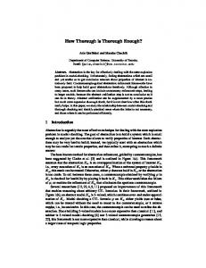
Schematic drawing of the simulation domain and the numerical mesh of 0.3125 × 0.30 mm elements for the steel bars of 0.0254 m diameter and 0.1 m length immersed in water and exchanging heat by a flux q during quenching.
of microconstituents weighted by their volume fractions. Note that, although the temperature field was calculated with AC3® to simulate the microstructure evolution, it was also calculated with Abaqus® by numerically solving the energy conservation equation, described below ∂T 1 ∂ ⎛ ∂T ⎞ ∂ ⎛ ∂T ⎞ 3 ∂fi = + + ∑Li ρC p rk k .... (2) ∂t r ∂r ⎜⎝ ∂r ⎟⎠ ∂z ⎜⎝ ∂z ⎟⎠ i =1 ∂t where t is time; ρ, Cp, and k are the steel density, specific heat, and thermal conductivity, respectively; Li is the volumetric latent heat of phase transformation from austenite to microconstituent i (Table 1), which in the present work can be pearlite, bainite, or martensite; and fi is the volume fraction of the microconstituent, obtained from AC3®. The summation on the right-hand side of Eq. (2) represents the total latent heat released during quenching as a result of phase transformations. The thermal conductivity, k, and specific heat, Cp, were calculated as averages of the corresponding properties of all microconstituents within each finite element, weighted by their volume fractions in the element. The thermal conductivities and specific heats of austenite, martensite, and bainite are given in Table 2. The volume fractions of these constituents for a specific location and temperature within the bar were interpolated in Abaqus® from the volume fractions calculated with AC3® at different radial positions. The heat transfer boundary condition at the bar surface was ∂T q = −k = h ( T − Tw ) + σε T 4 − Tw4 ........... (3) ∂n where q is the heat flux out of the bar; n is the direction normal to each part of the whole bar surface; σ is the StefanBoltzmann constant; and ε is the emissivity of the oxidized steel surface (ε = 0.76). Note that, in this equation, the heat flux by convection and radiation to the quenching water is accounted for. The same heat transfer coefficient used in the heat transfer simulations with AC3® was used in Abaqus® (see section 3). The initial condition was a uniform temperature field of 850°C inside the bar.
(
© 2014 ISIJ
)
term
⎛
∂f ⎞
∑ i =1 ⎜⎝ βi ∂Ti ⎟⎠ 3
cient, where βi =
to the average linear expansion coeffi-
α vi and α vi are respectively the linear 300
dilatation coefficient17,21,22) and the relative volumetric 1398
ISIJ International, Vol. 54 (2014), No. 6 Table 3. Young modulus and Poisson coefficient of austenite, martensite, bainite, and pearlite as function of temperature (°C).28–30) Constituent
Young modulus (GPa) –6×10⁻⁹T 3 + 6×10⁻⁶T 2 – 0.084T + 200
8×10–11T 3 – 7×10⁻⁸T 2 + 7×10⁻⁵T + 0.29
Martensite
–6×10⁻⁵T 2 – 0.033T + 200
8×10–11T 3 – 9×10⁻⁸T 2 + 7×10⁻⁵T + 0.28
Bainite
4×10⁻⁸T 3 – 3×10⁻⁵T 2 + 0.045T + 200
2×10–11T 3 – 3×10⁻⁸T 2 + 6×10⁻⁵T + 0.28
Pearlite
2×10⁻⁸T 3 – 0.0001T 2 + 0.016T + 200
2×10–11T 3 – 3×10⁻⁸T 2 + 6×10⁻⁵T + 0.28
Constituent
Steel
Poisson coefficient
Austenite
Table 4.
Table 5.
Chemical composition of the AISI 1045, 4140, and 4340 steel bars. Chemical Composition (%Mass) C
Cr
S
P
Mn
Mo
Ni
Si
AISI 1045
0.44 0.017 0.008 0.016 0.86 0.0007 0.0062 0.15
AISI 4140
0.39 1.01
0.025 0.018 0.87 0.17
0.12
0.17
AISI 4340
0.41 0.82
0.004 0.010 0.77 0.23
1.74
0.19
Yield and tensile strength of austenite, martensite, bainite, and pearlite as a function of temperature, T (°C).28–30) Yield strength (MPa) –8
3
–5
2
Tensile strength (MPa)
Austenite
31×10 T – 43×10 T + 0.05T + 299
3×10⁻⁷T 3 – 42×10–5T 2 – 44×10–3T + 373.7
Martensite
–0.001T 2 – 0.1T + 1 000
–103T 2 – 0.1T + 1 075
Bainite
10–9T 4 – 30×10–7T 3 + 18×10–4T 2 – 0.65T + 549
–9×10⁻⁷T 3 + 8×10⁻⁴T 2 – 0.5T + 624
Pearlite
–4×10⁻⁷T 3 + 56×10–5T 2 – 0.6T + 360
–4×10⁻⁷T 3 + 55×10–5T 2 – 0.6T + 435
expansion38) (Table 1) of microconstituent i (pearlite, bainite, or martensite), and
∂fi is the change in volume fraction of ∂T
this microconstituent per unit temperature variation, obtained from the microstructure evolution model. To define the boundary condition for the strain-stress simulations, the whole quenched bar surface was assumed free from forces or stresses. To carry out all the numerical simulations, a two dimensional axisymmetric model in cylindrical coordinates was used in Abaqus® (Fig. 1). The rectangular domain of the model was discretized by a mesh of CAX4T type elements (axisymmetric quadrilateral with 4 nodes and bilinear in displacement and temperature), containing 40 (r direction) × 333 (z direction) = 13 320 elements connected by 13 694 nodes at the element corners. To define this mesh, a refining test was conducted by comparing the calculated residual stresses for increasingly more refined meshes. As shown in section 5.3, the mesh with 13 320 elements provided a very good compromise between computational time and mesh independent results. The initial time step for the simulations was 0.01 s, but it was automatically adjusted by Abaqus® when necessary, changing in the range between 0.004 s and 0.1 s.
Fig. 2.
Schematic drawing of the cylindrical steel bar and its longitudinal section indicating the locations of the two sheathed thermocouples inserted to measured the cooling curves during quenching (dimensions are in mm).
latter case, two cooling curves were measured by inserting two type K (Chromel-Alumel) thermocouples at two different locations within the steel bar (Fig. 2). The thermocouple wires were insulated by compacted ceramic and sheathed by a stainless steel tube of 1.5 mm external diameter. These wires were connected to a data acquisition system that included a personal computer to collect the thermocouple signals at a rate of 10 s–1 and convert them into cooling curves. Each pair of cooling curves measured in one experiment was used to obtain, by an inverse solution technique, the heat transfer coefficient (h) between the surface of the steel bar and the quenching water. This coefficient was adopted to describe the boundary conditions in all heat transfer simulations with AC3® and Abaqus® (section 2). The measured cooling curves were used to inversely solve the heat conduction equation without the latent heat of phase transformation, which is Eq. (2) without the last term on the right-hand side. The latent heat was neglected during the inverse solution, because the microstructure evolution was still unknown at this step. During the final simulations of residual stresses, however, the complete Eq. (2) including the latent heat term was solved. The heat conduction equation was subject to the boundary condition given by Eq. (3), in which the value of h was unknown. The inverse solution technique consisted of a trial-and-error process in which different constant values of h were tested. For each value, the cooling curves were calculated with Abaqus® at the same position as those of the thermocouples and the total squared
3. Quenching Experiments and Calculation of Heat Transfer Coefficient Experimental results were obtained to validate the model described in section 2. Cylindrical bars of 0.0254 m diameter and 0.1 m length made of the three types of steels, namely, AISI 1045, 4140, and 4340 (Table 5) were first austenitized at 850°C for 1 h and subsequently quenched by immersion into a cylindrical tank (0.28 m diameter, 0.29 m depth) of water at the temperature of 24°C. During quenching, the bars were manually stirred by a continuous circular motion at approximately 96 rotations per minute. At least three quenching experiments were carried out for each steel grade under the same conditions: one for microstructural characterization, one for residual stress measurements, and the other for cooling curve measurements. In the 1399
© 2014 ISIJ
ISIJ International, Vol. 54 (2014), No. 6
The desired stress component, σφ , is calculated from the slope of the curve of 2θ as function of sin2ψ for X–ray beams incident on the surface in different orientations, being diffracted by atomic planes with normal vectors of different angles ψ in relation to the surface normal. As mentioned before, the normal vector to the atomic diffracting plane and the direction of σφ should form a vertical plane perpendicular to the sample surface. Since in the present work σφ was obtained in the axial (σ φ = σz) and tangential (σ φ = σθ) directions, this plane was parallel and then perpendicular to the axis of the bar, respectively. The angle φ is an angle between σφ and one of the principal directions of the stress tensor on the sample surface. Although this angle is unknown, it is not necessary to calculate σφ from Eq. (5). The diffraction angle measurements were carried out in a Rigaku Rint 2000 diffractometer with a chromium tube (CrKα = 0.2291 nm). The orientation of the diffracting atomic planes, ψ, changed from –50° to +50° in steps of 10 s by changing the orientation of the X-ray beam incident on the sample surface. For this variation in ψ, two times the diffraction angle, 2θ, changed from 154.1° to 157.7° in 0.2° steps with reference to the (211) crystallographic planes. The lateral surface of the cylindrical bars, on which the measurements were carried out, was ground with emery papers with grains up to 1 200 mesh before and after quenching to remove any sign of oxidation and coarse surface roughness.
error (SE) was obtained between the measured and calculated cooling curves as follows: 2
N
(
SE ( h ) = ∑∑ TMi , j − TCi , j ( h ) i =1 j =1
)
2
.............. (4)
where TM and TC are the measured and calculated cooling curves, respectively; i indicates either of the two thermocouple positions; and N is the number of temperature measurements made along the quenching time by the data acquisition system for each thermocouple. The final adopted value of h, representing the inverse solution, was one that gave the smallest SE. Generally h is a function of time, but very good agreement between calculated and measured cooling curves was obtained using a simple constant value h = 7 200 W m–2 K–1, adopted in all simulations, as discussed in section 5.1. 4. Characterization of Samples The cross section of the quenched bars was ground, polished, and chemically etched to reveal its microstructure. The section of the AISI 1045 carbon steel bar was etched first with Nital 2% (2 ml of HNO3 and 98 ml of ethyl alcohol) for 10 s and subsequently with Vilella (0.5 ml of picric acid, 2.5 ml of HCl, and 50 ml of C2H5OH) for 5 s. The AISI 4340 and 4140 low-alloy steels were etched with modified Le Pera,39) consisting of one part of 1% sodium metabissulfite (Na2S2O5) diluted in water and two parts of 4% picric acid (C6H3N3O7) diluted in ethyl alcohol. In the micrographs, the volume fractions of pearlite, bainite, and martensite at the surface and center of the bars were measured by the point count method. Following this method, a square mesh of 391 points was superimposed on the microstructure and the fraction of points within the specific constituent was manually counted according to the ASTM E562-02 standard.40) This fraction of points gives an estimate of the volume fraction of each constituent, which can be compared with the results of the simulations. The residual stresses formed in the middle length of the bars during quenching were measured on a ~3 mm2 region of the lateral cylindrical surface by the X-ray diffraction method.41–43) In this method, the normal component (σ φ) of the residual stress vector acting on planes perpendicular to the surface is calculated from measurements of the spacing between atomic planes in the crystal lattice of the surface grains. This calculation is possible because the spacing between planes is sensitive to the presence of residual stresses. During the measurement process, an X-ray beam of constant wavelength is incident on the sample surface with an orientation angle that changes in steps until a diffracted beam is obtained. When the incident beam is diffracted, the angle between the surface normal and the normal to the diffracting atomic planes is calculated and denoted as ψ. As usual, the angle of diffraction θ of these planes is the angle between the diffracted or incident beam and the diffracting atomic planes. The incident beam orientations in relation to the surface are chosen to guarantee that the normal to the diffracting atomic plane (given by ψ ) and the desired stress component σφ form a plane normal to the sample surface. In this case, the following equation can be written from a combination of elasticity theory for isotropic bodies and Bragg’s law of diffraction41) ⎡ 2 (1 + υ ) σ φ ⎤ 2 2θ = ⎢ ⎥ sin ψ + 2θ n ................. (5) ⎢⎣ E cot g θ n ⎥⎦ where θ n is the angle of diffraction for an atomic plane parallel to the surface (ψ =0); E (210 GPa) is the Young modulus, and υ (0.29) is the Poisson’s ratio. The numerical values used for these two parameters are those generally adopted for steels at room temperature.44–46) © 2014 ISIJ
5. Results and Discussion 5.1.
Analysis of Heat Transfer during Quenching Experiments The heat transfer coefficient between the steel bar surface and the quenching water was calculated by the inverse solution of the heat conduction equation using the cooling curves measured in two positions within the bar (Fig. 2). In Fig. 3(a), the measured cooling curves are shown for three repetitions of the same quenching experiment. The curves calculated with Abaqus® (Fig. 3(a)) for the constant heat transfer coefficient of h = 7 200 W m–2 K–1, which was the adopted value in all simulations with Abaqus® and AC3®, are in very good agreement with the measured cooling curves. A constant heat transfer coefficient indicates that a unique heat transfer mechanism prevailed during the whole quenching period, although in the pool boiling literature three stages are usually identified, namely, film boiling, nucleate boiling, and free convection.47,48) The heat transfer coefficient in simple forced convection flow was estimated in the present experiments using the relation presented by Churchill and Bernstein,49) adopting 1.2 m/s as the relative velocity of water (bar quenched in circular motion of radius 12 cm at ~ 96 rotations per minute) and thermophysical properties of water at the film temperature of 100°C. The calculated value was 6 600 W m–2 K–1, which is lower than that obtained from the inverse solution (7 200 W m–2 K–1). The larger value from the inverse solution can be explained by an enhanced heat transfer caused by the vapor bubbles observed during quenching, immediately after immersing the steel bar into the water. Since a constant heat transfer coefficient (suggesting a constant heat transfer regime) yielded very good agreement between calculated and measured cooling curves, the prevailing heat transfer regime might have been one near the transition between forced convection and nucleate boiling. The first derivative of the cooling curves measured at the bar center always displayed a peak of low cooling rate magnitude at the temperature of about 300°C, followed by a sharp peak of high cooling rate at the temperature of approximately 100°C, as illustrated in Fig. 3(b). Note that this sharp peak is caused by an abrupt decrease in temperature observed in the cooling curve at ~23 s (Fig. 3(a)). This 1400
ISIJ International, Vol. 54 (2014), No. 6 (a)
(b)
Fig. 3.
Fig. 4.
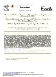
Heat transfer coefficient calculated in the present work and obtained by Fernandes and Prabhu52) as a function of the calculated surface temperature of the bar.
relatively low value probably owing to film boiling, increasing to ~ 8 000 W m–2 K–1, maybe as a result of nucleate boiling, approaching the present work constant value of 7 200 W m–2 K–1. The discrepancy between the h values at the beginning of quenching, for temperatures above 500°C, might be related to the higher agitation velocities in the present work. Higher velocities are known to disrupt the vapor blanket, eliminating the film boiling stage and consequently imposing nucleate boiling from the beginning of quenching.48) Another possible reason for the discrepancy can be seen in Fig. 3(a), showing that the surface temperature calculated with Abaqus® for the present samples decreased from 850 to 400°C in about 1 s. During this short period, only 10 temperature measurements were recorded by the data acquisition system. Therefore, in general, very few temperature measurements are available to calculate the heat transfer coefficient at the beginning of quenching, which is consequently more inaccurate during this first short initial period.
Cooling curves during quenching: (a) measured (Experiment) and calculated (Model) cooling curves at three different radial positions within the water-quenched bars in three experiments; and (b) the cooling curve measured at the center and its first derivative in relation to time (cooling rate) as a function of the measured bar center temperature.
5.2. Microstructural Evolution The micrographs of the three types of steels are given in Fig. 5 for the bar surface and in Fig. 6 for the bar center. The microstructure of the AISI 4340 steel is fully martensitic (Figs. 5(a) and 6(a)), while that of AISI 4140 shows martensite with some dark acicular bainite in both the surface (Fig. 5(b)) and center (Fig. 6(b)), but a larger volume fraction of martensite exists in the surface region owing to its higher cooling rate. For the AISI 1045 carbon steel, in addition to martensite and acicular bainite, some pearlite is also seen. The volume fraction of pearlite is larger at the bar center, because of the lower cooling rate (Fig. 6(c)). The microstructures in Figs. 5 and 6 show that, at corresponding bar regions, the amount of martensite increases in the studied steels in the order AISI 1045, 4140, and 4340, indicating an increasing hardenability as a result of the larger concentrations of alloying elements in this same order. The volume fractions of each microconstituent were measured at the center, mid-radius, and surface positions of the quenched bars by the point count method as described previously. Since the microstructure of the steel AISI 4340 was completely martensitic (Figs. 5(a) and 6(a)), the measurements were carried out only in the AISI 4140 and 1045 steels. The results are given in Table 6 and confirm the pre-
behavior was also observed in quenching experiments carried out by different authors8,50) and might be related to the latent heat released during the austenite to martensite phase transformation (Table 1), which occurs in this temperature range for the three types of steels examined in the present work.51) The heat transfer coefficient calculated in the present work was compared with that obtained by Fernandes and Prabhu52) in Fig. 4. Fernandes and Prabhu52) carried out lateral quenching experiments with 28 mm diameter AISI 1040 steel bars in water at Tw = 30°C, agitated at a velocity of ~0.3 m/s. These conditions are very similar to the present work conditions, except for the water velocity relative to the bar, which was estimated in the present work to be ~1.2 m/s at the beginning of the simultaneous quenching and stirring, decreasing to an unknown value as the water was dragged along during the circular motion of the bar within the water tank. The heat transfer coefficient (h) in the experiment of Fernandes and Prabhu52) was estimated from their reported surface heat flux (q) as a function of the surface temperature (Ts) using the equation h = q/(Ts – Tw). In Fig. 4, h from Fernandes and Prabhu52) is ~ 400 W m–2 K–1 at 850°C, a 1401
© 2014 ISIJ
ISIJ International, Vol. 54 (2014), No. 6 Table 6. Volume fractions (%) of martensite, bainite, and pearlite at the bar surface, mid-radius, and center for steels AISI 1045, 4140, and 4340. Fractions calculated with AC3® (model) and measured by the point counting method (exp) are given. Surface Steel
1045
Martensite
Mid-Radius
Bainite
Pearlite
Martensite
Bainite
Pearlite
Martensite
Bainite
Pearlite
Exp
Model
Exp
Model
Exp
Model
Exp
Model
Exp
Model
Exp
Model
Exp
Model
Exp
Model
Exp
Model
88
85
2.1
15
9.8
0
60
20
8.6
30
31
50
6.1
10
9.8
10
84
80
4140
90
95
4340
100
100
8.1
5
0
0
90
85
12
15
0
0
84
85
16
15
0
0
0
0
0
0
100
100
0
0
0
0
100
100
0
0
0
0
(a)
(a)
(b)
(b)
(c)
(c)
Fig. 5.
Center
Microstructure at the quenched bar surface for the three types of steels: (a) AISI 4340; (b) AISI 4140; and (c) AISI 1045. The microconstituents martensite (M), bainite (B), and pearlite (P) are indicated. (Online version in color.)
Fig. 6.
The microstructure evolution was modeled with AC3® using the calculated heat transfer coefficient of 7 200 W m–2 K–1, giving the volume fraction of all microconstituents as a function of time during quenching. The evolution of the calculated martensite volume fraction for the surface, mid-
vious qualitative analysis of the micrographs: the volume fractions of martensite increase from steel AISI 1045 to 4340. Furthermore, an increase in martensite is also observed from the center to the surface and this increase is larger for the 1045 owing to its lower hardenability. © 2014 ISIJ
Microstructure at the quenched bar center for the three types of steels: (a) AISI 4340; (b) AISI 4140; and (c) AISI 1045. The microconstituents martensite (M), bainite (B), and pearlite (P) are indicated. (Online version in color.)
1402
ISIJ International, Vol. 54 (2014), No. 6
The components of the residual stresses in the bar were calculated by the present model in the radial (σ r), tangential (σ θ), and axial (σ z) directions at the bar center and surface. These calculated values, shown in Table 7, represent the average value along a ~1 cm line of the domain boundary (bar surface or center), parallel to the bar axis. Before the
radius, and center positions of the 4340 steel is presented in Fig. 7. As expected, the largest calculated fraction is seen at the bar surface. At the end of quenching, as observed experimentally (Table 6), the structure is completely martensitic. In Table 6, measured and calculated volume fractions of microconstituents for the three types of steels are compared. This table shows that the best agreement occurs for the predictions of martensite volume fractions at the surface, midradius, and center of the two low-alloy steel bars. On the other hand, the largest discrepancies are observed in the fractions of all microconstituents for the AISI 1045 steel, especially at the mid-radius position.
(a)
5.3. Residual Stresses The diffraction angle, 2θ, as a function of sin2ψ (where ψ is the angle between the normal to the diffracting plane and the normal to the surface) obtained for the measurements of the axial (σz) and tangential (σθ) residual stresses on the surface of the AISI 4140 steel bar is given in Fig. 8. For each type of stress, there is one set of points for ψ > 0 and another for ψ < 0. It can be seen that the points lie approximately on a straight line, as predicted by Eq. (5), indicating accurate measurement procedures and good sample surface preparation. The two lines have approximately the same inclination, showing the absence of shear residual stresses at the surface. Similar curves of 2θ versus sin2ψ were obtained for all steel bars. As described in section 4, the measured axial and tangential residual stresses were obtained from the slope of these straight lines fitted to experimental points, as shown in Fig. 8 for the AISI 4140 steel. These measured stresses and their fitting errors are given in Table 7 for the three types of steels. Both tangential and axial surface residual stresses are compressive, in agreement with those reported by Lee and Lee.16) In their calculations and measurements for a quenched bar of an AISI 1045 steel, Inoue et al.17) obtained compressive tangential stresses that are larger than the axial stresses at the bar surface, as observed in the present work for the same type of steel (Table 7). Nevertheless, their values are about 30% of those in the present work. The smaller residual stresses obtained by these authors might be a result of the smaller bar diameter (20 mm diameter), resulting in less temperature gradient and more uniform plastic deformation, which usually decrease the magnitude of residual stresses.
(b)
Diffraction angle, 2θ, as a function of sin2ψ (where ψ is the angle between the surface normal and the normal to the diffracting plane) for the measurements of (a) axial, σz, and (b) tangential, σθ , residual stresses by the X-ray diffraction method on the surface of the AISI 4140 steel bar. Two sets of points were collected for the measurement of each type of stress, one for ψ > 0 and the other for ψ < 0.
Fig. 8.
Table 7.
Components of the residual stresses (MPa) measured experimentally (exp) at the bar surface and calculated (model) by the present finite element model at the bar surface and center: radial (σ r), tangential (σ θ), and axial (σ z) stress components.
Steel Radial (σr) center (model) Fig. 7.
Volume fraction of martensite calculated with AC3® as a function of time, at the surface, mid-radius and center positions of the AISI 4340 steel bar.
1403
Tangential (σθ) center surface (model) (model)
surface (exp)
Axial (σz) center surface (model) (model)
surface (exp)
1045
778
1 117
–286
–230 ± 20 1 128
–228
–206 ± 20
4140
892
784
–347
–360 ± 10 1 189
–329
–350 ± 20
4340
1 319
1 321
–391
–390 ± 50 1 848
–323
–350 ± 30
© 2014 ISIJ
ISIJ International, Vol. 54 (2014), No. 6
Fig. 9.
Fig. 10.
Calculated axial (σz), tangential (σθ), and radial (σr) residual stresses in the middle of the quenched AISI 4140 steel bar length as a function of the radial position from the bar center to the surface.
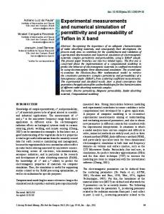
more pearlite, decreasing the yield strength and, therefore, decreasing the maximum possible magnitude of the residual stresses. Moreover, for the carbon steel, the difference between the time at which austenite begins to decompose at the surface and at the center is smaller, giving rise to lower residual stress originated from phase transformation. Maps of calculated σθ and σz in the simulation domain, which represents the longitudinal section of the bar indicated in Fig. 1, are given in Fig. 10, showing that, at the bar center, the axial tensile residual stresses (σ z) are always larger than the tangential stresses (σ θ), as also observed by several authors.15,53–56) The maps also show the distribution of residual stresses at the bar ends, which is significantly different from that at the middle length, being important to analyze the formation of quenching cracks. For example, the tangential stresses at the lateral surface change from compressive in the middle to tensile at the bar end, which could induce the formation of quenching cracks.
beginning of simulations, a mesh refining test was carried out to indicate the minimum number of mesh elements necessary for mesh independent results. In this test, σθ and σz at the cylinder surface were calculated using meshes successively refined from 1 660 to 53 360 elements. Finally, a mesh of 13 320 elements was chosen for all simulations, since further mesh refining did not change the calculated stresses significantly. The values of σθ and σz calculated at the bar surface are in reasonable agreement with the measured values (Table 7), generally showing discrepancies lower than 10%. Part of this discrepancy might be a result of neglecting the strain due to transformation plasticity in the model. The three calculated residual stress components (σr, σθ , and σz ) are tensile at the bar center, while at the bar surface σθ and σz are compressive, and σr is zero (not shown), as imposed by the boundary condition. The calculated residual stress profiles are shown in Fig. 9 for the AISI 4140 steel, changing continuously from tensile to compressive or zero when moving from center to surface, in agreement with stresses calculated by several authors.15,53–56) The measured and calculated residual stresses obtained in the present work can be explained by the following sequence of events described by Liscic57) and others:1,58) (a) there is axial and tangential thermal contraction of the bar surface during the initial cooling, creating thermal stresses that deform plastically the bar center in compression, while the surface is subjected to tensile stresses; (b) later, when the bar center cools significantly, its thermal contraction occurs, resulting in compressive stresses on the bar surface, i.e., reversing its stress state from tensile to compressive; (c) the decomposition of austenite occurs, causing a volume expansion first at the surface and later at the center. As explained by Liscic,57) when the austenite decomposition occurs after the stress reversal, its volume expansion does not change the stress sign caused by the thermal contraction/expansion, which would consequently be compressive at the surface and tensile at the center (Fig. 9), as observed in the present experiments and model results. The magnitude of both axial and tangential stresses generally increases from the carbon steel (AISI 1045) to the more alloyed steels (AISI 4140 and 4340), as seen in Table 7, which can be related to the microstructures described in Table 6. In the carbon steel there was less martensite and © 2014 ISIJ
Maps of the calculated tangential (σ θ) and axial (σ z) residual stresses in the simulation domain for the AISI 4140 steel bar, representing the longitudinal section indicated in Fig. 1. (Online version in color.)
6. Conclusions A mathematical model was implemented and experiments were carried out to investigate the build-up of residual stresses during water quenching of cylindrical carbon and low-alloy steel bars. The model is implemented using a combination of the commercial software packages AC3® and Abaqus® to simulate the different phenomena underlying the formation of residual stresses. Quenching experiments of cylindrical bars made of three types of steel grades, namely, AISI 1045, 4140, and 4340 were carried out to validate the proposed model. The heat transfer coefficient between the bars and the water during the quenching experiments is 7 200 W m–2 K–1, calculated by an inverse solution technique. Since this constant value (adopted in all simulations) results in very good agreement between calculated and measured cooling curves within the bars, approximately the same heat transfer regime must have prevailed during the experiments. This heat transfer coefficient is larger than that calculated for forced convection without boiling (6 600 W m–2 K–1), indicating that this constant heat transfer regime possibly corresponds to a transition between forced convection and nucleate boiling. In the observed microstructures of the bar cross sections, a larger volume fraction of martensite exists at the surface than at the center, as expected because of the larger surface 1404
ISIJ International, Vol. 54 (2014), No. 6
cooling rates. At the center and surface of the bars, the martensite fractions increase from the AISI 1045 to the 4140 steel, and finally to the 4340 steel, as a result of the higher hardenability of the low-alloy steels. The fractions of martensite calculated with the AC3® software are in good agreement with those measured in the low-alloy steels, but larger discrepancies are observed for all constituents in the midradius position of the carbon steel bar. Axial and tangential residual stresses measured on the surface (at middle length) of all quenched bars using the Xray diffraction method are compressive. These stresses increase from the carbon steel (AISI 1045) to the more alloyed steels (AISI 4140 and 4340) and are in good agreement with those calculated with the present model, showing discrepancies usually lower than 10%. Part of this discrepancy might be a result of neglecting the strain due to transformation plasticity in the model.
24) M. Sedighi and M. M. Salek: Trans. Can. Soc. Mech. Eng., 32 (2008), 1. 25) V. E. Scheil: Arch. Eisenhüttenwes., 8 (1935), 564. 26) M. Lusk and H.-J. Jou: Metall. Mater. Trans. A, 28 (1997), 287. 27) A. J. Fletcher: Thermal Stress and Strain Generation in Heat Treatment, Elsevier Applied Science, London, (1989), 92. 28) H. K. D. H. Bhadeshia: Handbook of Residual Stress and Deformation of Steel, ASM International, Materials Park, OH, (2002), 3. 29) R. Schröder: Mater. Sci. Technol., 1 (1985), 754. 30) R. Pietzsch, M. Brzoza, Y. Kaymak, E. Specht and A. Bertram: J. Appl. Mech., 74 (2007), 427. 31) H. Ghoneim: J. Therm. Stresses, 9 (1986), 345. 32) C. Heming, F. Jiang and W. Honggang: J. Mater. Process. Technol., 63 (1997), 568. 33) H. Cheng, J. Xie and J. Li: Comput. Mater. Sci., 29 (2004), 453. 34) E. P. Silva, P. M. C. L. Pacheco and M. A. Savi: Int. J. Solids Struct., 41 (2004), 1139. 35) G. S. Sarmiento, J. F. Bugna, L. C. F. Canale, R. M. M. Riofano, R. A. Mesquita, G. E. Totten and A. C. Canale: Mater. Sci. Eng. A, 459 (2007), 383. 36) S. Sen, B. Aksakal and A. Ozel: Int. J. Mech. Sci., 42 (2000), 2013. 37) R. Becker: Phys. Z., 26 (1925), 919. 38) K. E. Thelning: Steel and its Heat Treatment, Butterworths, London, (1975), 466. 39) G. A. Souza: Master Thesis, Department of Engineering, Universidade Estadual Paulista, São Paulo, Brazil, (2008), 161. 40) A. S. T. M. E562-02, Standard Test Method for Determining Volume Fraction by Systematic Manual Point Count, ASTM International, West Conshohocken, PA, (2002). 41) B. D. Cullity: Elements of X-Ray Diffraction, Addison-Wesley Publishing Company Inc, New York, (1978), 431. 42) P. S. Prevéy: X-Ray Diffraction Residual Stress Techniques, ASM International, Metals Park, OH, (1986), 380. 43) A. S. T. M. E1426-98, Standard Test Method for Determining the Effective Elastic Parameter for X-Ray Diffraction Measurements of Residual Stress, ASTM International, West Conshohocken, PA, (2009). 44) B. Coto, V. Navas, O. Gonzalo, A. Aranzabe and C. Sanz: Int. J. Adv. Manuf., 53 (2011), 911. 45) R. Menig, L. Pintschovius, V. Schulze and O. Vöhringer: Scr. Mater., 45 (2001), 977. 46) V. G. Navas, O. Gonzalo, I. Quintana and T. Pirling: Mater. Sci. Eng. A, 528 (2011), 5146. 47) F. P. Incropera, D. P. Dewitt, T. L. Bergman and A. S. Lavine: Fundamentals of Heat and Mass Transfer, John Wiley & Sons, New York, (2011), 619. 48) C. E. Bates, G. E. Totten, R. L. Brennan and E. F. Houghton: ASM Handbook - Heat Treating, ASM International, Materials Park, OH, (1991), 67. 49) S. W. Churchill and M. A. Bernstein: ASME Trans., 99 (1977), 300. 50) K. Babu and T. S. P. Kumar: J. Heat Transf., 133 (2011), 715011. 51) H. Chandler: Heat Treater’s Guide: Practices and Procedures for Irons and Steels, ASM International, Materials Park, OH, (1995), 904. 52) P. Fernandes and K. N. Prabhu: J. Mater. Process. Technol., 183 (2007), 1. 53) S. H. Kang and Y. T. Im: J. Mater. Process. Technol., 192 (2007), 381. 54) J. Grum, T. Kek, M. Zupancic, M. Batista and F. Kosel: Int. J. Microstruct. Mater., 3 (2008), 86. 55) S. Denis, P. Archambault, E. Gautier, A. Simon and G. Beck: J. Mater. Eng. Perform., 11 (2002), 92. 56) Y. Nagasaka, J. Brimacombe, E. Hawbolt, I. Samarasekera, B. Hernandez-Morales and S. Chidiac: Metall. Mater. Trans. A, 24 (1993), 795. 57) B. Liscic: Steel Heat Treatment – Metallurgy and Technologies, Taylor & Francis, Portland, (2007), 277. 58) P. Mayr: Dimensional Alteration of Parts due to Heat Treatment. In: Residual Stresses in Science and Technology, Vol. 1, GarmischPartenkirschen, DGM Informations-gesellschaft mbH, Federal Republic of Germany, (1987), 57.
Acknowledgements The authors thank Conselho Nacional de Desenvolvimento Científico e Tecnológico (CNPq) for the financial support (grants 134449/2010-0 and 310923/2011-5) and M. Sc. Juan Marcelo Rojas Arango for helping during measurements of the cooling curves. REFERENCES 1) G. E. Totten and N. A. Clinton: Handbook of Quenchants and Quenching Technology, ASM International, Materials Park, OH, (1993), 1. 2) D. Löhe, K. H. Long and O. Vöhringer: Handbook of Residual Stress and Deformation of Steel, ASM International, Materials Park, OH, (2002), 27. 3) C. S¸ims¸ir and C. H. Gür: Quenching and Cooling, Residual Stress and Distortion Control, ASM International, Materials Park, OH, (2010), 117. 4) M. Yaakoubi, M. Kchaou and F. Dammak: Comp. Mater. Sci., 68 (2013), 297. 5) S. N. Lingamanaik and B. K. Chen: Comp. Mater. Sci., 62 (2012), 99. 6) A. M. S. Hamouda, S. Sulaiman and C. K. Lau: J. Mater. Process. Technol., 119 (2001), 354. 7) M. Toparli, S. Sahin, E. Ozkaya and S. Sasaki: Comput. Struct., 80 (2002), 1763. 8) C. Heming, H. Xieqing and W. Honggang: J. Mater. Process. Technol., 90 (1999), 339. 9) P. Carlone and G. S. Palazzo: Int. Appl. Mech., 46 (2011), 955. 10) K. F. Wang, S. Chandrasekar and H. T. Y. Yang: J. Manuf. Sci. Eng., 119 (1997), 257. 11) C. S¸ims¸ir and C. H. Gür: Comp. Mater. Sci., 44 (2008), 588. 12) M. Ehlers, H. Muller and D. Lohe: J. Phys. IV, 9 (1999), 333. 13) B. L. Ferguson, Z. Liz and A. M. Freborg: Comp. Mater. Sci., 34 (2005), 274. 14) S. Jahanian and M. Mosleh: J. Mater. Eng. Perform., 8 (1999), 75. 15) L. Huiping, Z. Guoqun, N. Shanting and H. Chuanzhen: Mater. Sci. Eng. A, 452 (2007), 705. 16) S.-J. Lee and Y.-K. Lee: Acta Mater., 56 (2008), 1482. 17) T. Inoue, S. Nagaki, T. Kishino and M. Monkawa: Ing. Arch., 50 (1981), 315. 18) C. C. Liu, D. Y. Ju and T. Inoue: ISIJ Int., 42 (2002), 1125. 19) W. P. Oliveira, M. A. Savi, P. M. C. L. Pacheco and L. F. G. Souza: Mech. Mater., 42 (2010), 31. 20) T. Inoue and K. Arimoto: J. Mater. Eng. Perform., 6 (1997), 51. 21) T. Inoue, T. Tanaka, D. Y. Ju and R. Mukai: Key Eng. Mater., 345– 346 (2007), 915. 22) T. Inoue: Procedia Eng., 10 (2011), 3793. 23) S. Denis: J. Phys. IV, 6 (1996), 159.
1405
© 2014 ISIJ