Observer-Based State-Space Current Controller for a Grid Converter ...

This is an electronic reprint of the original article. This reprint may differ from the original in pagination and typographic detail.

Author(s):

Kukkola, Jarno & Hinkkanen, Marko & Zenger, Kai

Title:

Observer-Based State-Space Current Controller for a Grid Converter Equipped With an LCL Filter: Analytical Method for Direct Discrete-Time Design

Year:

2015

Version:

Post print

Please cite the original version: Kukkola, Jarno & Hinkkanen, Marko & Zenger, Kai. 2015. Observer-Based State-Space Current Controller for a Grid Converter Equipped With an LCL Filter: Analytical Method for Direct Discrete-Time Design. IEEE Transactions on Industry Applications. Volume 51, Issue 5. 4079-4090. ISSN 0093-9994 (printed). DOI: 10.1109/tia.2015.2437839. Rights:

© 2015 Institute of Electrical & Electronics Engineers (IEEE). Personal use of this material is permitted. Permission from IEEE must be obtained for all other uses, in any current or future media, including reprinting/republishing this material for advertising or promotional purposes, creating new collective works, for resale or redistribution to servers or lists, or reuse of any copyrighted component of this work in other work.

All material supplied via Aaltodoc is protected by copyright and other intellectual property rights, and duplication or sale of all or part of any of the repository collections is not permitted, except that material may be duplicated by you for your research use or educational purposes in electronic or print form. You must obtain permission for any other use. Electronic or print copies may not be offered, whether for sale or otherwise to anyone who is not an authorised user.

Powered by TCPDF (www.tcpdf.org)

IEEE TRANSACTIONS ON INDUSTRY APPLICATIONS

1

Observer-Based State-Space Current Controller for a Grid Converter Equipped With an LCL Filter: Analytical Method for Direct Discrete-Time Design Jarno Kukkola, Marko Hinkkanen, Senior Member, IEEE, and Kai Zenger, Member, IEEE

Abstract—State-space current control enables high dynamic performance of a three-phase grid-connected converter equipped with an LCL filter. In this paper, observer-based state-space control is designed using direct pole placement in the discrete-time domain and in grid-voltage coordinates. Analytical expressions for the controller and observer gains are derived as functions of the physical system parameters and design specifications. The connection between the physical parameters and the control algorithm enables automatic tuning. Parameter sensitivity of the control method is analyzed. The experimental results show that the resonance of the LCL filter is well damped, and the dynamic performance specified by direct pole placement is obtained for the reference tracking and grid-voltage disturbance rejection. Index Terms—Active damping, current control, grid-connected converter, LCL filter, parameter sensitivity, sensorless state feedback.

I. I NTRODUCTION

G

RID-CONNECTED converters play an important role in the grid integration of renewable energy sources. They are also increasingly used as an active front-end rectifier in motor drives, and interest for using an LCL filter between the converter and the grid has increased during the past few years. The LCL filter affords better grid-current quality, lower cost, and smaller physical size in comparison with the conventional L filter. However, a disadvantage of the LCL filters is the resonant behavior. The resonance can be damped actively using control [1] or passively at the expense of losses [2]. With state-space current control [3]–[12], the dominant and resonant dynamics can be simultaneously set through pole placement of the closedloop system. Hence, state-space control provides a convenient and straightforward way for resonance damping, when high dominant dynamic performance is desired [4].

Manuscript received November 20, 2014; revised February 10, 2015 and April 2, 2015; accepted April 25, 2015. Paper 2014-IPCC-0839.R2, presented at the 2014 IEEE Energy Conversion Congress and Exposition, Pittsburgh, PA, USA, September 20–24, and approved for publication in the IEEE T RANSAC TIONS ON I NDUSTRY A PPLICATIONS by the Industrial Power Converter Committee of the IEEE Industry Applications Society. This work was supported in part by ABB Oy and in part by the Walter Ahlström Foundation. The authors are with the Department of Electrical Engineering and Automation, Aalto University, 00076 Aalto, Finland (e-mail: [email protected]; [email protected]; [email protected]). Color versions of one or more of the figures in this paper are available online at http://ieeexplore.ieee.org. Digital Object Identifier 10.1109/TIA.2015.2437839

In state-space control, the closed-loop poles can be placed using various approaches: 1) dead-beat control [3]; 2) optimizing some cost function as in linear quadratic (LQ) control [3], [8], [9]; 3) using Bessel functions [5]; and 4) selecting the desired pole locations directly [4], [7], [10], [11]. LQ control is attractive for very complex systems, because it provides an indirect method for pole placement based on optimal control. However, the nonlinear Riccati equation has to be solved, which is not easy analytically or in real time. Furthermore, selection of the cost-function weights is difficult [9]. On the other hand, with direct pole placement, the controller gains can be analytically expressed using the parameters of the system and dynamic performance specifications (i.e., the bandwidth of current control and the resonance damping of the LCL filter) [4], [10], [11]. The analytical design methods enable automatic tuning and real-time adaptation of the controller, if the parameters are known or estimated. This is valuable in grid connection, because the topology and impedance of the grid can vary. The state-space current controller using direct pole placement has been analytically designed in stationary [4], [11] and synchronous coordinates [10]. When the state-space controller has been designed in stationary coordinates, current control has been implemented fully [4] or partially [11] in synchronous coordinates, and additional approximate cross-coupling compensation loops have been used. These loops are not needed, if the controller is directly designed in synchronous coordinates [10]. However, in [10], the continuous-time domain design has been used. Then, the controller must be discretized, which decreases feasible dynamic performance [13] and pole-placement accuracy with low sampling frequencies. The pole-placement accuracy in the direct discrete-time design is dependent on modeling accuracy. In [4], the design has been based on a model in stationary coordinates, although control has been implemented in synchronous coordinates. In [11], the crosscoupling compensation and integrator loops have been neglected in the pole-placement design. Thus, the pole-placement accuracy is decreased in [4] and [11]. In order to use statespace control, all the states must be measured or estimated [5], [7]–[10], [12], [14]. Direct discrete-time pole placement would be also a convenient method for tuning of the state observer, but no analytical solution in synchronous coordinates has been reported. In this paper, a discrete-time observer-based state-space current controller for the converter equipped with an LCL filter is

0093-9994 © 2015 IEEE. Translations and content mining are permitted for academic research only. Personal use is also permitted, but republication/redistribution requires IEEE permission. See http://www.ieee.org/publications_standards/publications/rights/index.html for more information.

2


Fig. 1. Space-vector circuit model of the LCL filter in stationary coordinates (marked with the superscript s).

coordinates rotating at the grid angular frequency ωg , the continuous-time dynamics of the converter current ic are ⎡ ⎤ ⎤ ⎡ 1 ⎤ ⎡ −jωg − L1fc 0 0 Lfc dx −jωg − C1f ⎦ x+ ⎣ 0 ⎦ uc + ⎣ 0 ⎦ ug = ⎣ C1f dt 1 − L1fg 0 −jωg 0 Lfg % &' ( % &' ( % &' ( Bc Bg ) *A 0 0 x. ic = 1 (1) &' ( % Cc

proposed. Due to the state observer, less sensors are needed in comparison with the methods in [3], [4], and [11]. The main contributions of this work are as follows. 1) Analytical expressions for the controller and observer gains are derived as functions of the physical filter parameters and the desired pole locations. Due to direct pole placement in synchronous coordinates, no additional cross-coupling compensation loops are needed. The analytical gain expressions enable implementation in real converters. 2) Design guidelines for selecting the pole locations are given. The effect of the varying grid impedance and LCL filter parameters on stability is examined. The proposed method is experimentally validated and compared with the design based on the continuous-time domain [10]. II. S YSTEM M ODEL Complex space vectors in synchronous dq coordinates are used (e.g., the converter current ic = icd + jicq ). Complex, matrix, and vector quantities are marked with boldface symbols. The equivalent circuit model for the LCL filter is shown in Fig. 1, and the state-space current control structure is shown in Fig. 2. Current control is implemented in grid-voltage oriented synchronous coordinates, where the grid voltage is ug = ug + j0. Two phase-to-phase grid voltages and the converter phase currents are measured for the state-space controller. Furthermore, the dc-link voltage ud is measured for the pulsewidth modulator (PWM), which calculates the duty cycles for the power switches. In the following, continuous-time and discrete-time LCL filter models for control design purposes are introduced. The losses of the filter are neglected for several reasons: 1) the lossless filter represents the worst case scenario for the resonance of the LCL filter; 2) the complexity of the discrete-time model and control algorithms will remain reasonable; and 3) particularly with higher power ratings, the losses in the filter are relatively small. A. Continuous-Time Model The state vector is selected as x = [ic , uf , ig ]T , where uf is the voltage across the filter capacitor Cf ; and ic and ig are the converter and grid currents, respectively. In synchronous

The transfer function from the converter voltage uc (s) to the converter current ic (s) is

where

Y(s) = Cc (sI − A)−1 Bc (s + jωg )2 + ωz2 1 * ) = Lfc (s + jωg ) (s + jωg )2 + ωp2 ωp =

+

Lfc + Lfg Lfc Lfg Cf

ωz =

+

1 Lfg Cf

(2)

(3)

are the resonance frequency and the antiresonance frequency of the filter, respectively. B. Hold-Equivalent Discrete-Time Model In the following, a hold-equivalent discrete-time model is presented. Sampling of the converter current and the grid voltage is synchronized with the PWM. The sampling frequency equals the switching frequency in the single-update PWM or twice the switching frequency in the double-update PWM. The switching-cycle-averaged converter output voltage is considered, and the PWM is modeled as the zero-order hold (ZOH) in stationary coordinates [15]. In other words, the converter voltage usc (t) is constant1 during kTs < t < (k + 1)Ts , where Ts is the sampling period, and k is the discrete-time index. On the contrary, the grid voltage ug (t) is assumed to be constant in synchronous coordinates during Ts . Furthermore, the filter parameters and the frequency ωg are assumed to be constant during the sampling period. Under these assumptions, the exact discrete-time model of (1) becomes x(k + 1) = Φx(k) + Γc uc (k) + Γg ug (k) ic (k) = Cc x(k)

(4)

where the system matrices are ⎛T ⎞ .s Φ = eATs , Γc = ⎝ eAτ e−jωg (Ts −τ ) dτ ⎠ Bc ⎛ 0T ⎞ .s Γg = ⎝ eAτ dτ ⎠ Bg .

(5)

0

1 If the reference for the PWM is updated in the middle of the sampling period, the averaged converter voltage is piecewise constant [16]. A discretetime model could be also derived for this particular scheme.

KUKKOLA et al.: STATE-SPACE CURRENT CONTROLLER FOR A GRID CONVERTER EQUIPPED WITH A FILTER

3

Fig. 2. Current control system. The gray blocks represent the plant model, and the white blocks represent the control algorithm. The sampling is synchronized with the PWM. The effect of the computational delay z −1 on the angle of the converter voltage usc is compensated for in the coordinate transformation. In the implementation, the grid-voltage angle ϑg and the magnitude ug are calculated using a PLL. In order to simplify the block diagram, the signal uc is fed directly ˆ d = [ˆ through the state observer block and included in its output vector, i.e., x xT uc ]T .

For Γc , the factor e−jωg (Ts −τ ) inside the integral originates from the ZOH being modeled in stationary coordinates, i.e., the converter voltage is time variant in synchronous coordinates during Ts . The closed-form expressions for the elements of the matrices in (5) are given in Appendix A. Due to the finite computation time, the converter-voltage reference usc,ref calculated at the present time step becomes active at the next time step. This delay is modeled in stationary coordinates as usc (k) = usc,ref (k − 1), when the PWM operates in the linear region. In synchronous coordinates, the relation is uc (k) = u′c,ref (k − 1) = e−jωg Ts uc,ref (k − 1), where the modified reference u′c,ref is introduced in order to simplify notation. The computational delay can be included in the discrete-time model as 1 2 1 2 1 2 Φ Γc 0 ′ Γ xd (k) + uc,ref (k) + g ug (k) xd (k + 1) = 0 0 1 0 % &' ( %&'( % &' ( Φd

Γcd

Γgd

* 0 xd (k) ic (k) = Cc % &' ( )

(6)

Cd

where kt is the feedforward gain, kI is the integral gain, K = ˆd = [ˆ x T , u c ]T [k1 , k2 , k3 , k4 ] is the state-feedback gain, and x is the state estimate augmented with the delayed voltage reference. A compensation for the angular displacement due to the computational delay is included in the coordinate transformation, as shown in Fig. 2. The state feedback together with the integral action can be designed from the standpoint of resonance damping and disturbance rejection. The reference feedforward provides an additional degree of freedom for the reference-tracking design. 2) Analytical Pole-Placement Design: For pole placement, the system model (6) is augmented with the integral state (7), resulting in 2 1 Φd xd (k + 1) = xI (k + 1) −Cd % &' ( % &' 1

xa (k+1)

Φa

Γca

1 2 1 2 0 Γgd + i (k) + ug (k) 1 c,ref 0 %&'( % &' ( Γra

where the new state vector is xd = [xT , uc ]T .

21 2 1 2 Γcd ′ 0 xd (k) uc,ref (k) + 1 xI (k) 0 % &' ( (

(9)

Γga

where xa is the augmented state vector; and Φa , Γca , Γra , and Γga are the augmented system matrices. From (8) and (9), the closed-loop dynamics become

III. C URRENT C ONTROL D ESIGN A. State-Space Controller 1) Control Law: The current control structure is shown in Fig. 2. For improved disturbance rejection, an integral state xI (k + 1) = xI (k) + ic,ref (k) − ic (k)

(7)

is introduced, where ic,ref is the reference current. The statespace control law is xd (k) u′c,ref (k) = kt ic,ref (k) + kI xI (k) − Kˆ

(8)

xa (k + 1) = (Φa − Γca Ka )xa (k) + (Γca kt + Γra )ic,ref (k) + Γga ug (k) ic (k) = Ca xa (k)

(10)

where Ka = [K, −kI ] is the augmented state-feedback gain, Ca = [1, 0, 0, 0, 0] is the output matrix, and the state estimate x ˆd in (8) has been replaced with the true state xd based on the

4


Fig. 3. Pole–zero plots. (a) Poles and zeros of the open-loop transfer function from u′c,ref (z) to ic (z). (b) Closed-loop poles are set to the desired locations. (c) Poles and zeros of the closed-loop transfer function from ic,ref (z) to ic (z).

separation principle [17]. The transfer function from the current reference ic,ref (z) to the converter current ic (z) is Gc (z) =

b(z) = Ca (zI − Φa + Γca Ka )−1 (Γca kt + Γra ). a(z) (11)

The numerator polynomial is b(z) = bc1 (z − β 1 )(z − β 2 )(kt z − kt + kI )

(12)

where bc1 is the first element of the input matrix Γc [cf., (26) in Appendix A], β 1 and β 2 are the resonant open-loop zeros, and the third zero depends on the feedforward gain kt . The denominator polynomial (i.e., the characteristic polynomial) is a(z) = det(zI − Φa + Γca Ka ).

(13)

Let the desired closed-loop characteristic polynomial be a(z) = z(z − α1 )(z − α2 )(z − α3 )(z − α4 )

(14)

where one pole originating from the computational delay is set to zero, and the selection of the four remaining pole locations will be discussed in Section III-A3. The gain Ka leading to the desired characteristic polynomial (14) could be solved using numerical tools. However, if the gain can be computed in the microprocessor of a converter, the control system can be tuned automatically, and the performance specifications can be changed in real time. For this purpose, analytical expressions for the gain Ka as a function of the system parameters and the desired pole locations are derived in Appendix B. 3) Selection of Pole Locations: Fig. 3(a) shows the poles and the zeros of the open-loop transfer function from u′c,ref (z) to ic (z), obtained from (6). The poles and zeros on the unit circle are the discrete counterparts of those in (2). Furthermore, there is a pole originating from the delay at z = 0. The poles of the closed-loop system can be arbitrarily set within the limits of the accessible control effort and modeling precision. When selecting pole locations, compromises between robustness and dynamic performance have to be made [4], [10]. In the characteristic polynomial (14), the two complex poles α1,2 are placed to determine the dominant dynamics

(i.e., the bandwidth), and the other two poles α3,4 are placed to determine the resonant dynamics (i.e., the resonance damping). It is typically easier to specify the pole locations first in the continuous-time domain and then map them to the discrete-time domain via z = exp(sTs ). In the continuous-time domain, the dominant and resonant dynamics can be split into two secondorder polynomials as 2 2 ) (s2 + 2ζcr ωcr s + ωcr ). (s2 + 2ζcd ωcd s + ωcd % &' (% &' ( Dominant dynamics

(15)

Resonant dynamics

Let us first consider the poles of the dominant dynamics. The natural frequency ωcd is related to the desired bandwidth, and the damping ratio is set to a high value, i.e., ζcd = 0.7, . . . , 1, in order to prevent large overshoots. The corresponding discrete poles are 13 5 2 4 2 ωcd Ts . (16) α1,2 = exp −ζcd ± j 1 − ζcd For simplicity, ζcd = 1 is selected here, leading to a double real pole. Fig. 3(b) illustrates the effect of the state-feedback control on the pole locations. The dominant complex pole at z = exp(−jωg Ts ) is moved to z = exp(−ωcd Ts ), and the pole originating from the integral state is also placed at z = exp(−ωcd Ts ), leading to a double real pole. To keep control effort low, the resonant pole pair should be kept near its natural frequency (i.e., ωcr ≈ ωp ). It is typically sufficient to damp the resonance with the ratio of ζcr = 0.1, . . . , 0.4. Selecting much higher values for ζcr is not recommended due to the increasing control effort [17]. The closedloop resonant poles are placed asymmetrically, i.e., 9 : 67 8 2 ω T (17) α3,4 = exp(−jωg Ts ) · exp −ζcr ± j 1 − ζcr cr s corresponding to the asymmetry of the open-loop resonant poles. Here, ζcr = 0.2 is selected. It is shown in Fig. 3(b) that the resonant poles are damped, but their frequency is not altered in order to minimize the control effort. Fig. 4 shows the frequency responses of the transfer function from the grid voltage ug (z) to the grid current ig (z) for the


5

Fig. 4. Frequency response of the transfer function from the grid voltage ug (z) to the grid current ig (z) in synchronous coordinates. The open-loop transfer function is obtained from (4) as Y g,OL (z) = Cg (zI − Φ)−1 Γg , where Cg = [0, 0, 1]. The closed-loop transfer function Y g,CL is obtained from (10) in a similar manner.

Fig. 5. Frequency response of the transfer function (11) from the current reference ic,ref (z) to the converter current ic (z) in synchronous coordinates. Different (solid lines) damping ratios ζcr and the case without the reference feedforward (kt = 0, dashed line) are shown.

open- and closed-loop cases. These transfer functions can be interpreted as converter output admittances, and they describe the effect of the grid-voltage disturbance on the grid current. The damping ratio in the closed-loop case is ζcr = 0.2. It can be seen that the resonance peaks are well damped by the state-feedback control. Furthermore, the closed-loop transfer function is low in the vicinity of the zero frequency (within the approximate bandwidth ωcd of the control), where the control is effective against the disturbances. 4) Selection of a Zero Location: Fig. 3(c) shows the poles and zeros of the closed-loop transfer function (11) from ic,ref (z) to ic (z). Generally, the state-feedback control has no effect on the zeros. The open-loop zeros β 1,2 shown in Fig. 3(a) are also present in the closed-loop system. However, the reference-feedforward path of the control law (8) produces a new zero in (11). If the zero is to be placed at βt , the feedforward gain becomes kt = kI /(1 − βt ).

(18)

This zero can be used to cancel (fully or partially) the closedloop pole originating from the integral state [17]. Here, the zero is placed on the double pole, i.e., βt = exp(−ωcd Ts ).

Fig. 6. Flowchart of current control tuning.

Hence, the resulting low-frequency reference-tracking dynamics become of the first order, with an approximate bandwidth of ωcd . Fig. 5 presents the frequency response of the transfer function (11). It can be seen that the reference feedforward increases the reference-tracking bandwidth. It is to be noted that the feedforward gain has no impact on the closed-loop disturbancerejection transfer function. The aforementioned guidelines for selecting the pole and zero locations will be used in the parameter sensitivity analysis (see Section IV) and in the experiments (see Section V). It is worth noticing that the pole locations could be further optimized. Fig. 6 illustrates the process of computing the controller gains. The closed-loop poles can be placed using basic arithmetics, and no nonlinear equations need to be solved, contrary to LQ control [9]. This enables automatic tuning of the controller, if the system parameters are known or estimated. It is to be noted that steps 1–3 in Fig. 6 need to be calculated only once (during the start-up of a converter), if the filter parameters are not changed. The reference tracking and disturbance rejection dynamics can be easily altered in real time by running steps 4–6.

6


TABLE I N OMINAL S YSTEM PARAMETERS

Fig. 7. Space-vector circuit model of an LCL filter connected to an inductive grid in stationary coordinates. The voltage u ˆg at the PCC is used in the control system. TABLE II T UNING E XAMPLE

B. State Observer The state observer is given by x ˆ(k + 1) = Φˆ x(k) + Γc uc (k) + Γg ug (k) + Ko [ic (k) − Cc x ˆ(k)]

(19)

where Ko = [ko1 , ko2 , ko3 ]T is the observer gain matrix. The characteristic polynomial of the estimation-error dynamics is ao (z) = det(zI − Φ + Ko Cc )

(20)

and the desired characteristic polynomial is ao (z) = (z − αo1 )(z − αo2 )(z − αo3 ).

A. Analysis The real observer dynamics become x ˆ(k + 1) = Φˆ x(k) + Γc uc (k) + Γg

(21)

Analytical expressions for the observer gain Ko as a function of the system parameters and the desired closed-loop poles are given in Appendix B. Again, the discrete-time poles of ao (z) can be mapped via its 2 ). continuous-time counterpart (s + αod )(s2 + 2ζor ωor s + ωor The real pole αod determines the dominant dynamics, and the complex-conjugate poles (parametrized via ωor and ζor ) are placed at a higher frequency. A rule of thumb to select the observer poles is to set them at least twice as fast as the controller dynamics [17]. Here, the real pole αod = 2ωcd is selected, and the complex-conjugate poles are placed at the resonance frequency ωor = ωp − ωg with the damping ratio ζor = 0.7. Then, the controller poles dominate the dynamic response. The Nyquist frequency 1/(2Ts ) determines the uppermost limit for the selection of the poles. IV. PARAMETER S ENSITIVITY The stiff grid and accurate filter parameter estimates were assumed in the control design. Fig. 7 shows an equivalent circuit model of an LCL filter connected to an inductive grid. In the following, the stability of the control system is studied taking into account a nonzero grid inductance. Furthermore, the real filter parameters differ from the nominal values given in Table I. The real filter parameters are marked with the prime. The grid inductance is denoted by Lg , and the voltage at the point of common coupling (PCC) is denoted by u ˆg . The voltage u ˆg is used in the control system (instead of ug , which is not accessible). The design parameters are given in Table II, and the pole locations correspond to (16) and (17). Nominal parameters are used in the control system.

Lg uf (k) + L′fg ug (k) Lg + L′fg

+ Ko [Cc x(k) − Cc x ˆ(k)]

(22)

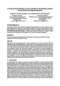
where uf = [0, 1, 0]x. The closed-loop dynamics, including the controller and the observer, consist of (8), (9), and (22), where the real parameters (L′fc , Cf′ , and L′fg + Lg ) are used in (9). The stability of the closed-loop system is analyzed considering three different cases: 1) the filter inductances are nominal: L′fc = Lfc and L′fg = Lfg ; 2) the filter inductances are 10% larger than the nominal values: L′fc = 1.1Lfc and L′fg = 1.1Lfg ; and 3) the filter inductances are 10% smaller than the nominal ones: L′fc = 0.9Lfc and L′fg = 0.9Lfg . In all the cases, the real filter capacitance Cf′ is varied from 0.5Cf to 1.5Cf , and the grid impedance Lg is varied from zero to Lfg . When Lg = Lfg , the effective grid-side inductance of the filter is doubled. The stability is examined by calculating the eigenvalues of the closed-loop system. Fig. 8 shows the regions where all the eigenvalues are inside the unit circle, i.e., the discrete system is stable. The figure illustrates also the regions where the damping ratios of all the eigenvalues are larger than 0.05. As shown in the figure, the example system is more sensitive to the parameter variations in the LCL filter than to the varying grid inductance Lg behind the PCC. If the manufacturing tolerance of 10% is considered for the filter components, the system remains stable within the examined range of the grid inductance Lg . Generally, the analysis predicts stable operation within a wide range of parameter variations. B. Simulations The parameter sensitivity analysis was validated using simulations. The dc voltage is constant, and the PWM of the converter was included in the model. A phase-locked loop (PLL) based on the synchronous-reference-frame transformation was


7

Fig. 8. Stability regions as a function of the relative capacitance Cf′ /Cf and grid inductance Lg /Lfg errors. Between the unity contours, all the eigenvalues of the closed-loop system are inside the unit circle (stable system). Between the dashed lines, the damping ratios of the eigenvalues are at least 0.05. Points marked by the crosses refer to the simulations in Fig. 9. (a) Real inductances in the LCL filter are nominal, i.e., L′fc = Lfc and L′fg = Lfg . (b) Real inductances are L′fc = 1.1Lfc and L′fg = 1.1Lfg . (c) Real inductances are L′fc = 0.9Lfc and L′fg = 0.9Lfg .

equipped with an LCL filter. The control method was implemented on the dSPACE DS1006 processor board. The switching frequency of the converter was 4 kHz, and synchronous sampling (twice per carrier) was used. The system parameters are given in Table I. The converter under test was regulating the dc-bus voltage at 650 V, whereas another back-toback connected converter was feeding the load to the bus. Synchronization was implemented with the PLL described in Section IV-B. A. Comparison Between the Proposed Method and Its Continuous-Time Counterpart

Fig. 9. Current step and grid-voltage dip responses, when the real system parameters are nominal (L′fc = Lfc , L′fg = Lfg , Cf′ = Cf , and Lg = 0) and changed (L′fc = 1.1Lfc , L′fg = 1.1Lfg , Cf′ = 1.1Cf , and Lg = Lfg ). Simulated (top) converter currents and (bottom) grid currents.

used for synchronization [18], and its closed-loop poles were set to the natural frequency of 2π · 20 rad/s with a damping √ ratio of 1/ 2. The reference icd,ref of the converter current was set to -10 A [-0.4 per unit (p.u.)], and the step of 10 A (0.4 p.u.) was applied in the reference icq,ref at t = 5 ms. A symmetric grid-voltage dip from 1 to 0.5 p.u. was applied at t = 15 ms. Fig. 9 shows simulation results for two cases: 1) the real filter parameters are nominal, and the grid is stiff; and 2) the real filter parameters differ from the nominal ones (L′fc = 1.1Lfc , Cf′ = 1.1Cf , and L′fg = 1.1Lfg ), and the grid inductance is Lg = Lfg . The simulated cases are also marked with the crosses in Fig. 8. The simulation results agree well with the analysis. The system is stable in both cases, but the resonance damping is lower, and the dominant dynamics are slightly slower in the case of parameter errors. It is to be noted that the analysis and simulations were carried out using the lossless LCL filter model; in practice, the losses increase damping. V. E XPERIMENTAL R ESULTS The proposed current control method was verified experimentally using a 12.5-kVA 400-V grid-connected converter

Tuning of the control system equals the tuning example introduced in Section IV-A and Table II. The proposed controller was experimentally compared with a corresponding observerbased state-space controller, which uses the same feedback information but is based on the continuous-time design [10]. The comparison was arranged as follows: 1) the same desired damping ratios were used; 2) the observer pole locations were equal in both methods under comparison; and 3) the dominant dynamics of the continuous-time design were tuned such that the converter-current rise time equaled that of the proposed design. Fig. 10 shows measured responses of the converter and grid currents, when a step of 10 A (0.4 p.u.) was applied in the converter current reference icq,ref . Approximately, the power of 5 kW (0.4 p.u.) was transferred through the converter leading to icd ≈ 10 A. It is to be noted that the grid currents were measured for monitoring purposes only and they were not used in the control. As the results show, the resonant dynamics are poorly damped in the case of the continuous-time design [10]. This is because the resonance frequency of 1.47 kHz is relatively high compared with the sampling frequency of 8 kHz, i.e., only a few samples are obtained during the period of the resonance frequency that should be damped. The controller designed in the continuous-time domain gives only an approximate mapping from the specified dynamics (the closedloop poles) to the controller gains and cannot fully treat the delays in the system. Hence, the realized dynamics are much worse than the desired dynamics. If the switching frequency (i.e., the sampling frequency) were increased or the specified

8


TABLE III H ARMONIC C OMPONENTS U NDER D ISTURBANCES

Fig. 11. Measured (top) grid voltage, (middle) grid currents, and (bottom) control errors of the converter current, when the grid voltage is distorted (ug5 = ug7 = 3%).

Fig. 10. Experimental comparison of the discrete-time (disc.) and continuoustime (cont.) control designs. Measured step responses. (a) Converter current components icd and icq . (b) Grid currents iga , igb , and igc .

bandwidth were lowered, the resonance damping of the continuous-time design [10] would be closer to the desired performance specifications. As shown in Fig. 10, the damping of the resonance frequency agrees well with the specified ratio ζcr = 0.2 in the case of the proposed discrete-time design. Moreover, the experimental results are in line with the corresponding analysis shown in Fig. 5 and the simulated results shown in Fig. 9. B. Operation During Grid Disturbances Disturbance rejection of the proposed method under gridvoltage harmonics and dips was experimentally evaluated. The distorted grid voltage was supplied using a 50-kVA three-phase four-quadrant power supply (Regatron TopCon TC.ACS). 1) Grid-Voltage Harmonics: The fifth and seventh harmonic components (ug5 and ug7 , respectively) were superimposed on the grid voltage. Three different harmonic levels (0%, 3%, and 5%) were tested. The converter was rectifying a power of 1 p.u. The grid currents iga , igb , and igc were monitored. In addition to the measurements, the same harmonic levels were simulated. The resulting harmonic currents ig5 and ig7 are given in Table III.

The total harmonic distortion (THD) of the grid current was calculated up to the 50th order. Without the harmonic disturbances, the THD is 1.6%, which is well below the 5% limit often given in standards (e.g., IEEE Std 519-2014 and IEEE Std 1547). Fig. 11 shows the grid currents and the control errors of the converter current in the case of the distorted voltage ug5 = ug7 = 3%. The harmonic components of the grid current conform to the aforementioned standards (ig5 < 4%, ig7 < 4%, and THD < 5%). When the harmonic level is increased to ug5 = ug7 = 5%, corresponding to the recommended maximum level in IEEE Std 519-2014, the current component ig7 is slightly over the 4% limit and THD > 5%. The measured harmonic components are also in line with the simulated components given in Table III. In order to improve the harmonic-disturbance rejection, the proposed control scheme could be augmented with resonant integrators in parallel with the existing integrator (cf., e.g., [4], [19], and [20]). 2) Grid-Voltage Dip: Disturbance rejection against the gridvoltage dip of 0.5 p.u. was evaluated. The converter was supplying the power of 0.4 p.u. to the grid. The measured responses of the grid currents and control errors of the converter current are shown in Fig. 12. As can be seen, the proposed method can reject the voltage dip well, and the cross-coupling between the error components is minor. Moreover, the measured error dynamics correspond to the designed dynamics. The slower mode in the dynamics of the grid currents originates from the dc-voltage control that is giving the references for the current controller. VI. D ISCUSSION The proposed method was analytically tuned assuming the lossless LCL filter. This assumption enables analytical control


9

proach enables automatic tuning and real-time adaptation of the controller, if the system parameters are known or estimated. The effect of varying parameters on the stability is examined. The results indicate that the proposed control scheme is less sensitive to variation of the grid inductance than variation of the LCL filter parameters. The method is validated by means of simulations and experiments. The results show that higher dynamic performance and better resonance damping can be achieved with the proposed design in comparison with statespace control designed in the continuous-time domain. The results also show that the resonance of the LCL filter is well damped, and the dynamic performance specified by direct pole placement is obtained for the reference tracking and gridvoltage disturbance rejection. Fig. 12. Measured (top) grid voltage, (middle) grid currents, and (bottom) control errors of the converter current, when a grid-voltage dip is applied.

tuning, and it represents the worst case scenario for the resonance of the LCL filter. The experimental results were shown for a low-power converter equipped with an LCL filter that has relatively higher losses in comparison with filters designed for higher power ratings (reaching megavoltampere ratings). As shown by the results, the accuracy of the lossless model is adequate in order to achieve desired dynamic performance. On the other hand, the simulation models were lossless. Thus, it can be concluded that the proposed method is valid for lossless filters (or low-loss filters) as well. This is valuable in the case of the higher power ratings, where both the losses and switching frequencies tend to be lower. The accurate parameter estimates and the stiff grid voltage have been assumed in the control design. In these ideal conditions, the current-control dynamics do not couple with the PLL dynamics. Naturally, the stable current-control loop in the ideal conditions is a practical precondition for the stability of the entire control system. In weak grids, current control together with the PLL may cause converter–grid or converter–converter interactions leading to oscillations or instability [19], [21]–[24]. In order to mitigate the oscillations, the output impedance of the converter has been shaped [21]. Since the current-control bandwidth is typically high in comparison with outer control loops, current control has an impact on the output impedance in a wide range of frequencies. Since the proposed control method is flexible, it could be used to shape the converter output impedance via its design parameters. Moreover, the degrees of freedom equal those of the methods in [3] and [4], but less sensors are needed because of the state observer. The number of the sensors could be further decreased by replacing the grid-voltage measurement with estimation as in [7], [8], and [25]–[27]. VII. C ONCLUSION This paper has presented a direct discrete-time design method for an observer-based state-space current controller of a grid converter equipped with an LCL filter. Model-based pole placement in synchronous coordinates is used to derive an analytical control design. Contrary to LQ control, the proposed ap-

A PPENDIX A H OLD -E QUIVALENT D ISCRETE -T IME M ODEL The state transition matrix Φ in (4) can be calculated, e.g., using eigendecomposition A = PΛP−1 , where the eigenvector and eigenvalue matrices are ⎡

−Lfg /Lfc P = ⎣ −jωp Lfg 1

⎤ −Lfg /Lfc jωp Lfg ⎦ 1

1 0 1

(23)

Λ = diag {−j(ωg + ωp ), −jωg , −j(ωg − ωp )} . With this decomposition, the matrix exponential is Φ = eATs = PeΛTs P−1 , where the exponential of the diagonal matrix can be calculated elementwise. The result is ⎡

a11 Φ = ⎣a21 a31 ⎡ =γ

⎤ a13 a23 ⎦ a33

a12 a22 a32

Lfc +Lfg cos(ωp Ts ) Lt ⎢ sin(ωp Ts ) ⎢ ω p Cf ⎣ Lfc [1−cos(ωp Ts )] Lt

−

⎤

Lfg [1−cos(ωp Ts )] Lt ⎥ sin(ω T ) ⎥ − ωp Cp f s ⎦ Lfg +Lfc cos(ωp Ts ) Lt

sin(ωp Ts ) ωp Lfc

cos(ωp Ts ) sin(ωp Ts ) ωp Lfg

(24)

where γ = e−jωg Ts , and Lt = Lfc + Lfg . The input matrix for the converter voltage (5) is ⎛

Γc = P ⎝

.Ts 0

⎞

eΛτ e−jωg (Ts −τ ) dτ ⎠ P−1 Bc .

(25)

The resulting input matrix for the converter voltage is ⎡ Ts Lfg sin(ωp Ts ) ⎤ ⎤ bc1 Lt + ωp Lfc Lt ⎢ p Ts )] ⎥ Γc = ⎣bc2 ⎦ = γ ⎣ Lfg [1−cos(ω ⎦. Lt sin(ωp Ts ) Ts bc3 − ⎡

Lt

ω p Lt

(26)

10


Using similar calculations, coefficients of the input matrix for the grid voltage Γg = [bg1 , bg2 , bg3 ]T in (5) become

where pi , q i , r i , si , and ti (i = 0, . . . , 3) are functions of the system parameters p0 = f 3 a11 + f 4 a21 + f 5 a31

bg1

) * γ −ωg ωp sin(ωp Ts ) + jωg2 cos(ωp Ts ) − jδ − jωp2 = δωg (Lfc + Lfg )

bg2

γ [ωp cos(ωp Ts ) + jωg sin(ωp Ts )] − ωp = δωp Cf Lfg

s0 = f 7 bc1 + (a11 a32 − a12 a31 )bc2 − f 1 bc3

bg3 = γ

+

jωg2 Lfc

ωg ωp Lfc sin(ωp Ts ) − jδLfg − δωg Lfg (Lfc + Lfg )

(27)

s1 = − s0 − a31 bc1 − a32 bc2 + (a11 + a22 )bc3

(32)

q 2 = − (a22 + a33 + 1)bc1 + a12 bc2 + a13 bc3

r 2 = − (a11 + a33 + 1)bc2 + a21 bc1 + a23 bc3 s2 = − (a11 + a22 + 1)bc3 + a31 bc1 + a32 bc2 t2 = bc1

The desired characteristic polynomial (14) is expressed as (28)

where the coefficients as functions of the pole locations are a 1 = α1 α2 α3 α4

p3 = − a11 − a22 − a33 − 1 q 3 = bc1 ,

r 3 = bc2 ,

(33) (34)

s3 = bc3

where the auxiliary parameters are f 1 = a11 a22 − a12 a21 ,

f 2 = a11 a33 − a13 a31

f 3 = a22 a33 − a23 a32 ,

f 4 = a13 a32 − a12 a33

f 5 = a12 a23 − a13 a22 ,

f 6 = a21 a33 − a23 a31

f 7 = a22 a31 − a21 a32 .

a2 = − α 1 α 2 α 3 − α 1 α 2 α 4 − α 1 α 3 α 4 − α 2 α 3 α 4

(35)

Equating (28) and (30) directly gives the gain

a3 = α 1 α 2 + α 1 α 3 + α 1 α 4 + α 2 α 3 + α 2 α 4 + α 3 α 4 (29)

Analytical expressions for the state-feedback gain Ka as a function of the system parameters and the desired coefficients ai are derived in the following. The discrete-time system parameters aij , bci , and bgi (i, j = 1, . . . , 3) are given in (24), (26), and (27), respectively. The determinant in (13) is calculated, leading to a(z) = det(zI − Φa + Γca Ka ) = z 5 + (k4 − a22 − a33 − a11 − 1)z 4 + (p3 k4 + q 3 k1 + r 3 k2 + s3 k3 + p2 )z 3 + (p2 k4 + q 2 k1 + r 2 k2 + s2 k3 + t2 kI + p1 )z 2 + (p1 k4 + q 1 k1 + r 1 k2 + s1 k3 + t1 kI + p0 )z + p0 k 4 + q 0 k 1 + r 0 k 2 + s 0 k 3 + t0 k I

r 1 = − r 0 − a21 bc1 + (a11 + a33 )bc2 − a23 bc3

p2 = a11 + a22 + a33 + f 1 + f 2 + f 3

A. State-Feedback Gain

a4 = − α 1 − α 2 − α 3 − α 4 .

p 1 = − p0 − f 1 − f 2 − f 3

t1 = − (a22 + a33 )bc1 + a12 bc2 + a13 bc3

A PPENDIX B A NALYTICAL G AIN E XPRESSIONS

a0 = 0,

(31)

q 1 = − q 0 + (a22 + a33 )bc1 − a12 bc2 − a13 bc3

where δ = ωg2 − ωp2 .

a(z) = z 5 + a4 z 4 + a3 z 3 + a2 z 2 + a1 z + a0

r 0 = f 6 bc1 − f 2 bc2 + (a11 a23 − a13 a21 )bc3 t0 = f 3 bc1 + f 4 bc2 + f 5 bc3

cos(ωp Ts )

jδLfg + jωg2 Lfc δωg Lfg (Lfc + Lfg )

q 0 = − f 3 bc1 − f 4 bc2 − f 5 bc3

(30)

k4 = a4 + a11 + a22 + a33 + 1

(36)

and, furthermore, a system of four linear equations, i.e., ⎡ ⎤ ⎤⎡ ⎤ ⎡ q0 a0 − p0 k 4 r0 s0 t0 k1 ⎢q 1 ⎢ ⎥ ⎢ ⎥ r1 s1 t1 ⎥ ⎢ ⎥ ⎢k2 ⎥ = ⎢a1 − p1 k4 − p0 ⎥ (37) ⎣q 2 r2 s2 t2 ⎦ ⎣k 3 ⎦ ⎣ a 2 − p 2 k 4 − p 1 ⎦ q3 r3 s3 0 kI a 3 − p3 k 4 − p2 &' ( % &' ( % &' ( % K′

M

W

where (36) has been used. The remaining gains could be solved using matrix inversion K′ = M−1 W. In real-time systems, it is more efficient to solve the gains using the following steps. 1) The mapping matrix M = LU is expressed using the LU decomposition as ⎤ ⎤⎡ ⎡ u12 u13 u14 1 0 0 0 u11 ⎢ ⎢l21 1 0 0⎥ u22 u23 u24 ⎥ ⎥. ⎥⎢ 0 M=⎢ ⎣ ⎦ ⎣l31 l32 1 0 0 0 u33 u34 ⎦ l41 l42 l43 1 0 0 0 u44 % &' (% &' ( L

U

(38)


2) Equating (37) and (38) gives the elements of the lower diagonal matrix L, i.e., l21 = q 1 /q 0 l41 = q 3 /q 0 ,

l31 = q 2 /q 0 ,

l32 = (r 2 − l31 r 0 )/u22

l42 = (r 3 − l41 r 0 )/u22 (39)

l43 = (s3 − l41 s0 − l42 u23 )/u33 and of the upper diagonal matrix U, i.e., u11 = q 0 u13 = s0 ,

u12 = r 0 ,

u23 = s1 − s0 l21

u24 = t1 − t0 l21 ,

ko1 = ao2 + a11 + a22 + a33 ko2 = [f 5 (ao1 − f 1 − f 2 − f 3 + a22 ko1 + a33 ko1 ) − a13 (ao0 + a11 f 3 − a12 f 6 − a13 f 7 − f 3 ko1 )] /(a12 f 5 − a13 f 4 ) ko3 = (ao0 + a11 f 3 − a12 f 6 − a13 f 7 − f 3 ko1 − f 4 ko2 )/f 5 (44)

R EFERENCES u14 = t0

u34 = t2 − l31 t0 − l32 u24

u44 = − l41 t0 − l42 u24 − l43 u34 .

(40)

3) The decomposition enables calculation of the gains from LUK′ = W by solving two back-substitution problems: LC = W and UK′ = C. The elements of the auxiliary vector C = [c0 , c1 , c2 , c3 ]T are obtained by solving the first back-substitution problem C = L−1 W, i.e., c0 = w 0 ,

Analytical expressions for the observer gains as a function of the system parameters and the desired coefficients are

where the auxiliary parameters f i are given in (35).

u22 = r 1 − r 0 l21

u33 = s2 − l31 s0 − l32 u23 ,

11

c1 = w1 − l21 c0

c2 = w2 − l31 c0 − l32 c1 , c3 = w3 − l41 c0 − l42 c1 − l43 c2

(41)

where wi are the elements of W = [w0 , w1 , w2 , w3 ]T in (37). 4) The second back-substitution problem K′ = U−1 C gives the gains kI = c3 /u44 k3 = (c2 − u34 kI )/u33

(42)

k2 = (c1 − u23 k3 − u24 kI )/u22 k1 = (c0 − u12 k2 − u13 k3 − u14 kI )/u11 . These steps were also applied in the real-time implementation in Section V. If the filter parameters and performance specifications are constant, these gains need to be calculated only once (during the start-up of a converter). B. Observer Gain The desired coefficients of the characteristic polynomial (21) as functions of the desired pole locations are ao0 = − αo1 αo2 αo3 ao1 = αo1 αo2 + αo1 αo3 + αo2 αo3 ao2 = − αo1 − αo2 − αo3 .

(43)

[1] V. Blasko and V. Kaura, “A novel control to actively damp resonance in input LC filter of a three-phase voltage source converter,” IEEE Trans. Ind. Appl., vol. 33, no. 2, pp. 542–550, Mar./Apr. 1997. [2] R. Peña-Alzola et al., “Analysis of the passive damping losses in LCLfilter-based grid converters,” IEEE Trans. Power Electron., vol. 28, no. 6, pp. 2642–2646, Jun. 2013. [3] E. Wu and P. W. Lehn, “Digital current control of a voltage source converter with active damping of LCL resonance,” IEEE Trans. Power Electron., vol. 21, no. 5, pp. 1364–1373, Sep. 2006. [4] J. Dannehl, F. W. Fuchs, and P. B. Thøgersen, “PI state space current control of grid-connected PWM converters with LCL filters,” IEEE Trans. Power Electron., vol. 25, no. 9, pp. 2320–2330, Sep. 2010. [5] C. Ramos, A. Martins, and A. Carvalho, “Complex state-space current controller for grid-connected converters with an LCL filter,” in Proc. IEEE IECON, Porto, Portugal, Nov. 2009, pp. 296–301. [6] I. J. Gabe, V. F. Montagner, and H. Pinheiro, “Design and implementation of a robust current controller for VSI connected to the grid through an LCL filter,” IEEE Trans. Power Electron., vol. 24, no. 6, pp. 1444–1452, Jun. 2009. [7] M. Xue et al., “Full feedforward of grid voltage for discrete state feedback controlled grid-connected inverter with LCL filter,” IEEE Trans. Power Electron., vol. 27, no. 10, pp. 4234–4247, Oct. 2012. [8] B. Bolsens, K. De Brabandere, J. Van den Keybus, J. Driesen, and R. Belmans, “Model-based generation of low distortion currents in gridcoupled PWM-inverters using an LCL output filter,” IEEE Trans. Power Electron., vol. 21, no. 4, pp. 1032–1040, Jul. 2006. [9] F. Huerta et al., “LQG servo controller for the current control of LCL gridconnected voltage-source converters,” IEEE Trans. Ind. Electron., vol. 59, no. 11, pp. 4272–4284, Nov. 2012. [10] J. Kukkola and M. Hinkkanen, “Observer-based state-space current control for a three-phase grid-connected converter equipped with an LCL filter,” IEEE Trans. Ind. Appl., vol. 50, no. 4, pp. 2700–2709, Jul./Aug. 2014. [11] M. H. Hedayati, B. A. Acharya, and V. John, “Common-mode and differential-mode active damping for PWM rectifiers,” IEEE Trans. Power Electron., vol. 29, no. 6, pp. 3188–3200, Jun. 2014. [12] V. Miskovic, V. Blasko, T. M. Jahns, A. H. C. Smith, and C. Romenesko, “Observer-based active damping of LCL resonance in grid-connected voltage source converters,” IEEE Trans. Ind. Appl., vol. 50, no. 6, pp. 3977–3985, Nov./Dec. 2014. [13] R. Turner, S. Walton, and R. Duke, “Robust high-performance inverter control using discrete direct-design pole placement,” IEEE Trans. Ind. Electron., vol. 58, no. 1, pp. 348–357, Jan. 2011. [14] N. Hoffmann, M. Hempel, M. C. Harke, and F. W. Fuchs, “Observer-based grid voltage disturbance rejection for grid connected voltage source PWM converters with line side LCL filters,” in Proc. IEEE ECCE, Raleigh, NC, USA, Sep. 2012, pp. 69–76. [15] H. Kim, M. W. Degner, J. M. Guerrero, F. Briz, and R. D. Lorenz, “Discrete-time current regulator design for ac machine drives,” IEEE Trans. Ind. Appl., vol. 46, no. 4, pp. 1425–1435, Jul./Aug. 2010. [16] N. Hoffmann, F. W. Fuchs, and J. Dannehl, “Models and effects of different updating and sampling concepts to the control of grid-connected PWM converters—A study based on discrete time domain analysis,” in Proc. EPE 2011, Birmingham, U.K., Sep. 2011, pp. 1–10. [17] G. F. Franklin, J. D. Powell, and M. Workman, Digital Control of Dynamic Systems. Menlo Park, CA, USA: Addison-Wesley, 1997. [18] V. Kaura and V. Blasko, “Operation of a phase locked loop system under distorted utility conditions,” IEEE Trans. Ind. Appl., vol. 33, no. 1, pp. 58–63, Jan./Feb. 1997.

12


[19] L. Harnefors, A. G. Yepes, A. Vidal, and J. Doval-Gandoy, “Passivitybased controller design of grid-connected VSCs for prevention of electrical resonance instability,” IEEE Trans. Ind. Electron., vol. 62, no. 2, pp. 702–710, Feb. 2015. [20] M. Liserre, R. Teodorescu, and F. Blaabjerg, “Multiple harmonics control for three-phase grid converter systems with the use of PI-RES current controller in a rotating frame,” IEEE Trans. Power Electron., vol. 21, no. 3, pp. 836–841, May 2006. [21] L. Harnefors, M. Bongiorno, and S. Lundberg, “Input-admittance calculation and shaping for controlled voltage-source converters,” IEEE Trans. Ind. Electron., vol. 54, no. 6, pp. 3323–3334, Dec. 2007. [22] J. H. R. Enslin and P. J. M. Heskes, “Harmonic interaction between a large number of distributed power inverters and the distribution network,” IEEE Trans. Power Electron., vol. 19, no. 6, pp. 1586–1593, Nov. 2004. [23] X. Wang, F. Blaabjerg, and W. Wu, “Modeling and analysis of harmonic stability in an ac power-electronics-based power system,” IEEE Trans. Power Electron., vol. 29, no. 12, pp. 6421–6432, Dec. 2014. [24] J. Sun, “Impedance-based stability criterion for grid-connected inverters,” IEEE Trans. Power Electron., vol. 26, no. 11, pp. 3075–3078, Nov. 2011. [25] S. Mariéthoz and M. Morari, “Explicit model-predictive control of a PWM inverter with an LCL filter,” IEEE Trans. Ind. Electron., vol. 56, no. 2, pp. 389–399, Feb. 2009. [26] M. Malinowski and S. Bernet, “A simple voltage sensorless active damping scheme for three-phase PWM converters with an LCL filter,” IEEE Trans. Ind. Electron., vol. 55, no. 4, pp. 1876–1880, Apr. 2008. [27] J. Kukkola and M. Hinkkanen, “State observer for grid-voltage sensorless control of a grid-connected converter equipped with an LCL filter,” in Proc. EPE-ECCE Eur., Lappeenranta, Finland, Aug. 2014, pp. 1–10.

Marko Hinkkanen (M’06–SM’13) received the M.Sc.(Eng.) and D.Sc.(Tech.) degrees from Helsinki University of Technology, Espoo, Finland, in 2000 and 2004, respectively. Since 2000, he has been with Helsinki University of Technology (part of Aalto University, Espoo, since 2010). He is currently an Assistant Professor with the School of Electrical Engineering, Aalto University. His research interests include control systems, electric drives, and power converters.

Jarno Kukkola received the B.Sc.(Tech.) and M.Sc.(Tech.) degrees from Aalto University, Espoo, Finland, in 2010 and 2012, respectively, where he is currently working toward the D.Sc.(Tech.) degree in the School of Electrical Engineering. His main research interests include grid-connected converters.

Kai Zenger (M’07) received the M.Sc. degree in electrical engineering, the L.Sc. degree in computer technology, and the D.Sc. degree in automation and systems technology from Helsinki University of Technology, Espoo, Finland, in 1986, 1992, and 2003, respectively. From 1983 to 1989, he was an Automation Engineer with MKT Finland and HT Automation. Since 1989, he held several positions related to teaching and research in the Control Engineering Laboratory, Helsinki University of Technology, Espoo, Finland. He is currently a Senior Lecturer of automation technology with the School of Electrical Engineering, Aalto University, Espoo. His main research areas are, in general, control engineering and systems theory, with applications in chemical process engineering, electrical engineering, power electronics, and mechanical engineering. He has specialized in research of time-varying linear systems, periodic systems, and adaptive and robust control methods.